Shape Optimization
Shape Optimization: Theoretical Foundations
Shape Optimization
Professor, how is shape optimization different from topology optimization?
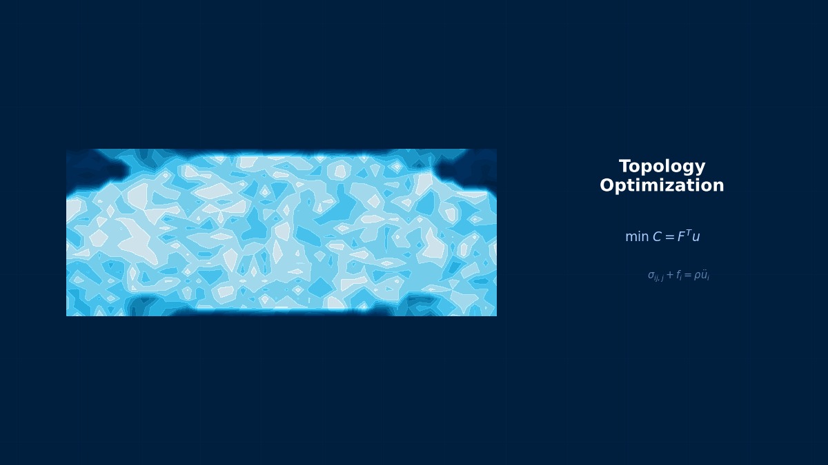
Topology optimization is about "whether to create or keep holes." Shape optimization fine-tunes existing boundaries (external shapes). It optimizes fillet radii or curved surface shapes without changing the number of holes.
$$ \min_{\mathbf{x}_{boundary}} f(\mathbf{x}_{boundary}) \quad \text{s.t.} \quad g_i \leq 0 $$
Professor, how is shape optimization different from topology optimization?
Topology optimization is about "whether to create or keep holes." Shape optimization fine-tunes existing boundaries (external shapes). It optimizes fillet radii or curved surface shapes without changing the number of holes.
The design variables are the nodal coordinates of the boundary surface. Sensitivity is calculated to move the boundary.
Summary
The Partial Differential Equation for Shape Optimization is Formulated Using the Calculus of Variations
The mathematical foundation of shape optimization lies in the Calculus of Variations. Céa (1986) formulated the first variation of the objective function with respect to shape change—the "Shape Gradient"—as the weak form of a partial differential equation, which became the cornerstone of finite element method-based shape optimization. The method of numerically integrating the shape gradient on the boundary (Boundary Integral Method) is computationally efficient and has versatility, applicable uniformly from fluid drag minimization (Stokes equations) to structural stress minimization (elasticity equations).
Computational Methods for Shape Optimization
FEM for Shape Optimization
Abaqus TOSCA Shape: Moves nodes on the design surface in the normal direction. Improves the objective function using sensitivity (Adjoint Method). Updates shape via mesh morphing.
Summary
Free-Form Shape Optimization (FFD) Originates from Pixar's Imaging Technology
Free-Form Deformation (FFD) is a computer graphics technique developed by Sederberg and Parry, presented at SIGGRAPH in 1986, evolving from Barr's (1984) deformation model. The technology used for character facial deformation in Pixar's animated film "Toy Story (1995)" was repurposed in the 2000s as mesh deformation technology in Ansys Fluent and OpenFOAM, becoming a standard tool for wing shape optimization. Public literature shows that FFD-based SU2 was utilized for the winglet shape optimization of the Airbus A350.
Shape Optimization in Practice
Practical Shape Optimization
Fillet optimization (stress concentration reduction), wall thickness distribution optimization for castings.
Practical Checklist
Bicycle Frame Shape Optimization Updated TT Record by 7 Seconds
The fork and chainstay shapes of the Looke Sport Science TT bike ridden by Bradley Wiggins at the 2012 London Olympics were optimized using NSGA-II-based shape optimization (using Solidworks Flow Simulation), reducing the frame's aerodynamic drag from CD=0.28 to 0.21. The development team announced this corresponded to a 7-second time reduction on a 10km TT course. It is now industry standard for top road racing equipment brands to apply CFD shape optimization to all their models.
Shape Optimization: Software & Solver Comparison
Tools
CADDESS's SCARS Specializes in F1 Car Aerodynamic Shape Optimization
UK-based CADDESS's SCARS is a shape optimization tool specialized for SPLINE parametric optimization of profile shapes, with adoption records in F1 team wing shape design. Racecar Engineering magazine (2018) reported that MercedesAMG Petronas F1 uses a shape optimization loop combining SCARS and Star-CCM adjoint sensitivity for front wing development. In sports car and aircraft exterior design, Ansys Discovery Shape is also a competitor, featuring real-time shape sensitivity display that designers can operate intuitively.
Advanced Technologies
Advanced Shape Optimization
Pioneer of Shape Optimization: History of CEA CAD Integration
Engineering application of shape optimization accelerated after Bendsøe and Kikuchi proposed topology optimization in 1988, when France's CEA applied a shape optimization system linking parametric CAD and sensitivity analysis to nuclear reactor containment vessel design. In modern ANSYS Mechanical + SpaceClaim integration, the functionality to directly reflect sensitivity information onto NURBS control points is
Related Topics
Experience the theory firsthand with the interactive simulator for this field
All Simulators