Rayleigh-Bénard convection
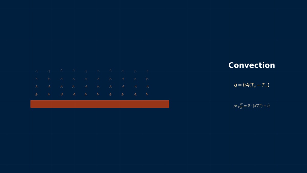
Theory: rest or convection
Overview
When you heat a pan of water gently, the warm water at the bottom doesn't rise straight away. Is there some trigger?
There is. A layer that is warm below and cool above has heavy fluid on top, which is unstable, but viscosity and thermal diffusion act as brakes. For a small temperature difference the fluid stays still and heat crosses by conduction alone. The moment buoyancy beats the brakes, the fluid organises into rolls and starts moving all at once. The Rayleigh number sets that threshold — about 1708 between two solid walls. That is Rayleigh–Bénard convection.
Rayleigh number and its critical value
| Boundaries | Critical Ra | Critical wavenumber $a_c$ |
|---|---|---|
| Rigid–rigid | 1707.8 | 3.117 |
| Rigid–free | 1100.7 | 2.682 |
| Free–free | 657.5 | 2.221 |
$H$ is the layer depth and $\Delta T$ the temperature difference. At onset the roll wavelength is about $2H$, so each roll is roughly as wide as the layer is deep. Because Ra scales with $H^3$, doubling the depth multiplies it by eight.
Bénard's hexagons were not caused by buoyancy
In 1900 Henri Bénard reported neat hexagonal patterns on the surface of a thin heated liquid layer. In 1916 Lord Rayleigh explained such instability through buoyancy, and the phenomenon took both names. But Bénard's layers were very thin with a free upper surface, and later work — Pearson in 1958 among others — showed the main driver there was surface tension varying with temperature (the Marangoni effect). It is a rare case where the name and the physics never quite matched.
Worked example: air-gap thickness and heat flux
Nusselt number of an air layer
For a horizontal air layer heated from below, the correlation of Hollands et al. (1975) is widely used ($[\,]^+$ means zero when negative):
Results for air at 300 K ($\nu = 1.59\times10^{-5}$ m²/s, $\alpha = 2.25\times10^{-5}$ m²/s, $k = 0.0263$ W/(m·K)) with a 10 K temperature difference:
| Gap | Ra | Nu | Heat flux |
|---|---|---|---|
| 5 mm | 114 | 1.00 | 52.6 W/m² |
| 10 mm | 915 | 1.00 | 26.3 W/m² |
| 15 mm | 3,087 | 1.64 | 28.8 W/m² |
| 20 mm | 7,317 | 2.18 | 28.7 W/m² |
| 30 mm | 24,695 | 2.96 | 25.9 W/m² |
| 50 mm | 114,328 | 4.12 | 21.6 W/m² |
A 15 mm gap loses more heat than 10 mm! I assumed thicker always insulates better.
With conduction alone, heat flux falls in inverse proportion to thickness. Here convection starts at about 12 mm and cancels most of the benefit of going thicker. That is why air gaps in double glazing and insulated panels have an optimum thickness. For vertical layers such as windows convection behaves differently, so use the correlations for natural convection in enclosures.
Water convects far more readily
For a 50 mm layer of water at 20 °C ($\nu = 1.0\times10^{-6}$ m²/s, $\alpha = 1.43\times10^{-7}$ m²/s, $\beta = 2.07\times10^{-4}$ 1/K), a mere 1 K difference gives a Rayleigh number of about $1.8\times10^{6}$ — a thousand times critical. Assuming liquid in a tank or battery coolant stays still “because the temperature difference is tiny” is risky.
How the flow changes with Rayleigh number
| Approximate Ra | Flow |
|---|---|
| Below 1708 | At rest; conduction only (Nu = 1) |
| 1708 to a few ×10⁴ | Steady two-dimensional rolls |
| About 10⁴ to 10⁶ | Rolls become three-dimensional and time-dependent |
| Higher | Turbulent: thin thermal boundary layers at the walls shedding plumes |
The transition values depend on the Prandtl number and the container aspect ratio, so treat the table as a rough guide.
Reproducing it correctly in CFD
Key setup points
- Buoyancy model: the Boussinesq approximation is fine for small temperature differences, roughly when $\beta\Delta T$ is well below 0.1. Beyond that, treat density as a function of temperature.
- Initial perturbation: with a perfectly uniform initial temperature and symmetric geometry, the numerical solution may stay in the conduction state. Add a small random perturbation of about 0.1% to the initial temperature.
- Solve in time: well above onset the flow fluctuates, so a steady solver either fails to converge or settles into one arbitrary state. Run transient and evaluate the Nusselt number averaged over a long enough time.
- Lateral extent: rolls are about as wide as the layer is deep, so the domain width dictates how many rolls fit. Use periodic sides or make the domain several depths wide.
Mesh that resolves the thermal boundary layers
Heat passes through thin thermal boundary layers at the top and bottom walls, so without cells there the Nusselt number will be wrong. As a guide, refine toward the walls so that several cells fall within $\delta_T$ estimated above. At $Nu = 10$, $\delta_T$ is only 5% of the depth.
How to verify
- Solve near onset — say Ra = 1500 and 2000 — and check that the flow decays back to Nu = 1 at 1500 and grows at 2000.
- At Ra = $10^4$–$10^5$, compare the time-averaged Nusselt number with the correlation above; within 10–20% is reasonable.
- Confirm the Nusselt number no longer changes with mesh refinement before moving to the real geometry.
Where weather-forecast chaos began
In 1963 the meteorologist Edward Lorenz was studying a three-variable system of differential equations — an extreme simplification of Rayleigh–Bénard convection — when he noticed that tiny differences in the initial values changed the outcome completely. That observation led to the discovery of chaos, popularly known as the butterfly effect. When convection CFD shows different instantaneous flow patterns from run to run under the same conditions, it is not a bug but this very property. Compare time-averaged quantities, not snapshots.
Common mistakes
Mistakes and fixes
| Mistake | Effect | Fix |
|---|---|---|
| Starting from a perfectly uniform state | No convection even above onset | Add a small perturbation to the initial temperature |
| Using the same correlation with the heated surface on top | The layer is stably stratified, so no convection; heat transfer overestimated | Treat top heating as conduction (Nu ≈ 1) |
| Applying horizontal-layer correlations to vertical layers | Convection behaves differently; large errors | Use enclosure correlations that include aspect ratio |
| Taking a steady-state result at face value | Only one arbitrary state of a fluctuating flow is captured | Run transient and time-average |
| Coarse mesh near the walls | Nusselt number badly off | Put several cells inside $\delta_T$ |
I'd like to change the parameters and watch convection start.
With the convection cells simulator you can vary the temperature difference and depth and find where rolls appear. For the dimensionless groups see the Grashof number simulator and the article on Grashof and Rayleigh numbers; for surface heat-transfer estimates, the natural convection coefficient calculator. The chaos Lorenz found can be explored with the Lorenz attractor simulator.
Related Topics
Experience the theory firsthand with the interactive simulator for this field
All Simulators