Adjust upstream velocity, pipe diameter, and fluid density to visualize pressure distribution in a Venturi tube with diameter-ratio sensitivity and device comparison across three real-time charts.
About Bernoulli's Principle Applications Simulator
🙋
I learned Bernoulli's theorem as "P + ½ρv² = const", but does the pressure really drop when the pipe is constricted? Intuitively, it doesn't quite click...
🎓
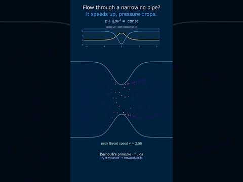
To get a feel for it, try pinching a shower hose. When you pinch it, the water comes out faster, right? That's exactly Bernoulli's theorem. When the pipe narrows, the continuity equation (A₁v₁ = A₂v₂) tells us the flow velocity increases. Then, from Bernoulli's theorem, the pressure drops. Roughly speaking, it's a "pay pressure to gain speed" relationship. Try reducing the "Throat Diameter D₂" in this tool—you'll see the pressure drop ΔP value go up steadily.
🙋
I see! But in actual factory piping, what is this pressure drop used for?
🎓
Flow measurement. For example, in water treatment plants or chemical factories, you want to know in real time how much liquid is flowing. So, you install a Venturi tube in the pipe and measure the pressure at two points—upstream and at the throat—with pressure gauges. From that difference (ΔP), you can calculate the flow rate using Q = Cd·A₂·√(2ΔP/ρ·A₁²/(A₁²-A₂²)). If you look at the "Device Comparison" tab in this tool, you can see at a glance how the accuracy (Cd) and pressure loss differ among Venturi tubes, flow nozzles, and orifice plates.
🙋
Looking at the "Diameter Ratio Sensitivity Analysis" tab, ΔP increases sharply as the diameter ratio gets larger. Why does it increase quadratically?
🎓
From the continuity equation, v₂ = v₁·(A₁/A₂) = v₁·(D₁/D₂)². Since the pressure drop is ΔP = ½ρ(v₂²-v₁²), and v₂ increases with the square of the diameter ratio, ΔP is proportional to v₂², so it effectively increases with the fourth power of (D₁/D₂)! For example, if the diameter ratio doubles, ΔP can theoretically increase by a factor of 16. So, "the narrower you make it, the higher the sensitivity," but in practice, you can't increase the diameter ratio indefinitely due to cavitation (a phenomenon where pressure drops below the saturation vapor pressure, causing bubbles to form). Design is all about this balance.
🙋
In the "Device Comparison" tab, there's a column called "Permanent Pressure Loss." What does that mean?
🎓
A Venturi tube has a shape that gradually expands after the throat, so most of the pressure that dropped at the throat recovers downstream. On the other hand, an orifice plate is a thin hole plate, so after the constriction, the flow expands abruptly, causing turbulence, and energy is lost as heat—this is the "permanent pressure loss." Venturi tubes are expensive but have low loss, leading to lower running costs (pump power). For large-diameter pipes in long-term plant operation, choosing a Venturi makes sense even with higher initial investment. Orifice plates are cheap and are often used when you need to measure at dozens of points in a factory.
🙋
I see, it's about cost-effectiveness. When I change the "Fluid Density" slider, ΔP also changes. When I calculate with air (about 1.2 kg/m³), ΔP becomes much smaller than with water. Does that have any important meaning?
🎓
Good observation! Since ΔP = ½ρ(v₂²-v₁²), the smaller the density ρ, the smaller the pressure difference for the same velocity difference. Air (ρ≈1.2) is about 1/833 of water (ρ≈1000), so using the same Venturi shape with air gives a ΔP only 1/833 of that with water. This is one reason why high-sensitivity hot-wire anemometers or ultrasonic flowmeters are used for air velocity measurement (airflow measurement). Conversely, for high-pressure gases (large ρ) or supersonic flows, compressibility can no longer be ignored, and the incompressible flow assumption of today's simulator breaks down—that's also the limit line of Bernoulli's theorem.
Physical Model & Key Equations
For steady, incompressible, inviscid flow, Bernoulli's theorem states that the following energy relation holds along a streamline.
$$P + \frac{1}{2}\rho v^2 + \rho g h = \text{const.}$$
For a horizontal pipe with no elevation change, $P_1 + \tfrac{1}{2}\rho v_1^2 = P_2 + \tfrac{1}{2}\rho v_2^2$, so static pressure decreases as velocity increases. $P$ : static pressure [Pa], $\rho$ : density [kg/m³], $v$ : velocity [m/s], $h$: elevation [m].
Combining it with the continuity equation from conservation of mass gives the velocity and pressure at each section.
Actual flow meters correct the volume flow rate using a discharge coefficient $C_d$ (Venturi≈0.98, nozzle≈0.95, orifice≈0.61).
How to Use the Three Tabs
📈 Pipe pressure and velocity distribution: Shows axial profiles for velocity (blue) and static pressure (red) along the Venturi tube. Velocity rises and static pressure drops sharply in the throat region (position 0.35-0.60), then pressure recovers in the diffuser.
🔬 Diameter-ratio sensitivity: Overlays ΔP-v₁ curves for fixed D₁/D₂ ratios of 2.0, 3.0, and 4.0. The yellow point marks the current setting, making the fourth-power nonlinearity of ΔP easy to see.
📊 Device comparison: Compares measured ΔP, permanent pressure loss, and discharge coefficient Cd for a Venturi tube, flow nozzle, and orifice. Changing upstream velocity or pipe diameter updates the bars and shows the tradeoffs under each condition.
Frequently Asked Questions
What is Bernoulli's principle?
For steady, incompressible, inviscid flow, P + ½ρv² + ρgh = const holds along a streamline. When a pipe is constricted, the continuity equation increases velocity, and Bernoulli's principle reduces static pressure. Conversely, expansion reduces velocity and recovers pressure. This 'speed-pressure trade-off' is the basis for flow meters, Pitot tubes, and wing lift.
How do you calculate flow rate in a Venturi tube?
Combine the continuity equation A₁v₁ = A₂v₂ with Bernoulli's equation, and use the pressure difference ΔP to find v₂ (velocity at the throat). The practical formula is Q = Cd·A₂·√(2ΔP / ρ·(1-(A₂/A₁)²)) (Cd is the discharge coefficient, about 0.98 for Venturi). By reading ΔP with a pressure gauge, the flow rate can be calculated instantly.
Explain the principle and usage of a Pitot tube.
A Pitot tube faces the fluid, locally reducing velocity to zero (stagnation point) and measuring total pressure (= static pressure + dynamic pressure). The difference from separately measured static pressure gives dynamic pressure q = ½ρv², and velocity is found as v = √(2q/ρ). It is used in aircraft airspeed indicators, wind tunnel velocity measurements, and chimney exhaust gas velocity measurements.
What are the differences between an orifice, nozzle, and Venturi tube?
All are differential pressure flow meters, but differ in shape and characteristics. Orifice (Cd≈0.61): thin plate, cheap and easy to install, but high pressure loss. Flow nozzle (Cd≈0.95): nozzle shape, moderate loss, good for slurries. Venturi (Cd≈0.98): gradual contraction and expansion, excellent pressure recovery, minimal permanent loss, long and expensive. For large flow pipes in long-term operation, Venturi is economical.
Under what conditions does Bernoulli's principle not hold?
Caution is needed under these conditions: ① High viscous losses (low Reynolds number, long pipes) — the Darcy-Weisbach friction loss term must be added to the energy equation. ② High-speed flow where compressibility is not negligible (Ma > 0.3). ③ Unsteady flow (e.g., water hammer from rapid valve opening/closing). ④ Two-phase flow (gas-liquid mixture). In these cases, more advanced fluid dynamics models are required.
What is the relationship between cavitation and pressure drop?
When static pressure at the Venturi throat drops below the liquid's saturation vapor pressure at that temperature, the liquid locally boils and forms bubbles (cavities) — this is cavitation. The bubbles collapse downstream, generating shock waves that erode walls and cause vibration and noise. A larger diameter ratio lowers throat pressure more easily, increasing cavitation risk. During design, the cavitation index (σ) is checked for margin.
What is Bernoulli Applications?
Bernoulli Applications is a fundamental topic in engineering and applied physics. This interactive simulator lets you explore the key behaviors and relationships by directly manipulating parameters and observing real-time results.
By combining numerical computation with visual feedback, the simulator bridges the gap between abstract theory and physical intuition — making it an effective learning tool for students and a rapid-verification tool for practicing engineers.
Physical Model & Key Equations
The simulator is based on the governing equations behind Bernoulli's Principle Applications. Understanding these equations is key to interpreting the results correctly.
Each parameter in the equations corresponds to a slider in the control panel. Moving a slider changes the equation's solution in real time, helping you build a direct connection between mathematical expressions and physical behavior.
Real-World Applications
Engineering Design: The concepts behind Bernoulli's Principle Applications are applied across mechanical, structural, electrical, and fluid engineering disciplines. This tool provides a quick way to estimate design parameters and sensitivity before committing to full CAE analysis.
Education & Research: Widely used in engineering curricula to connect theory with numerical computation. Also serves as a first-pass validation tool in research settings.
CAE Workflow Integration: Before running finite element (FEM) or computational fluid dynamics (CFD) simulations, engineers use simplified models like this to establish physical scale, identify dominant parameters, and define realistic boundary conditions.
Common Misconceptions and Points of Caution
Model assumptions: The mathematical model used here relies on simplifying assumptions such as linearity, homogeneity, and isotropy. Always verify that your real system satisfies these assumptions before applying results directly to design decisions.
Units and scale: Many calculation errors arise from unit conversion mistakes or order-of-magnitude errors. Pay close attention to the units shown next to each parameter input.
Validating results: Always sanity-check simulator output against physical intuition or hand calculations. If a result seems unexpected, review your input parameters or verify with an independent method.
Enter upstream velocity (v1) in m/s—typical range 0.5–15 m/s for pipe flow applications
Input upstream diameter (D1) and downstream diameter (D2) in millimeters; the simulator calculates area ratio automatically
Set fluid density (rho) in kg/m³—use 1000 for water, 860 for mineral oil, 1.2 for air at sea level
Click Calculate to solve for downstream velocity, pressure drop, and flow rate using continuity equation and Bernoulli's theorem
Worked Example
Water (ρ=1000 kg/m³) flows through a horizontal venturi tube. Upstream: D1=50 mm, v1=3 m/s, P1=200 kPa. Downstream: D2=25 mm. Continuity equation gives v2=12 m/s (area reduction by 4:1). Bernoulli's equation yields P2≈128 kPa, demonstrating 72 kPa pressure drop as velocity increases. Flow rate Q=A1×v1=0.00196×3=5.89 L/s.
Practical Notes
Venturi meters in hydraulic systems use this pressure-velocity relationship for flow measurement; maintain laminar conditions (Re<2300) for accuracy
Cavitation risk increases when P drops below vapor pressure (~2.3 kPa for water at 20°C); ensure downstream diameter doesn't exceed design limits