Visualize 2D potential flow around a cylinder with streamlines and pressure coefficient (Cp) color maps. Experience the Magnus effect and d'Alembert's paradox.
Flow Type
Parameters
Free-stream velocity U∞ (m/s)
m/s
Cylinder radius R
m
Circulation Γ (m²/s)
m²/s
Flow rate Q (+source / −sink)
m²/s
Display
Results
Results
0.000
Lift coeff. CL
0.000
Drag coeff. CD
−3.000
Cp (top, θ=90°)
−3.000
Cp (bottom, θ=270°)
Flow
Low Cp (fast)High Cp (slow)
Click on the canvas to inspect local velocity and Cp
Top: streamlines + Cp color map | Bottom: surface Cp distribution (θ = 0° → 360°)
What exactly is "potential flow" around a cylinder? It sounds abstract.
🎓
Basically, it's a simplified model for a smooth, inviscid (frictionless) fluid flowing past an object. In this simulator, the object is a cylinder. The "potential" part means the flow is irrotational, so we can describe it with a neat mathematical function. Try setting the Circulation (Γ) to zero and moving the "Free-stream velocity" slider above. You'll see perfectly symmetric streamlines wrapping around the cylinder.
🙋
Wait, really? But real air has friction. Why is this model useful if it ignores viscosity?
🎓
Great question! It's a foundational building block. For many high-speed or streamlined flows away from surfaces, viscous effects are small. More importantly, it gives us exact solutions to benchmark against and helps us understand lift generation. For instance, add some Circulation (Γ) now. See how the flow asymmetry creates a pressure difference? That's the core of lift on a spinning ball or an airfoil.
🙋
Okay, I see the streamlines curving. What does the "Flow rate Q" parameter do? Is that like adding a hose to the cylinder?
🎓
Exactly! A positive Q models a source—fluid magically appearing at the center, like a spring. A negative Q is a sink—fluid disappearing. This lets us model more complex shapes. In practice, combining a source, sink, and uniform flow can model flow around an oval-like body. Try a small positive Q and watch how the streamlines are pushed outward, as if the cylinder is blowing air.
Physical Model & Key Equations
The flow is defined by a stream function, Ψ. Its value is constant along a streamline. For flow around a cylinder with circulation, it combines uniform flow, a doublet (to create the cylinder), and a vortex (for circulation).
$$ \Psi(r,\theta) = U_\infty r \left(1-\frac{R^2}{r^2}\right) \sin\theta - \frac{\Gamma}{2\pi} \ln r $$
Where:
• $U_\infty$ = Free-stream velocity (m/s) – the wind speed far away.
• $R$ = Cylinder radius (m).
• $r, \theta$ = Polar coordinates from the cylinder's center.
• $\Gamma$ = Circulation (m²/s) – the strength of the swirling motion.
• The term with $\ln r$ is the vortex contribution, which breaks the flow symmetry.
The most powerful result is the Kutta-Joukowski theorem. It tells us that for any body in a potential flow, the lift force per unit length is directly proportional to the circulation.
$$ L = \rho U_\infty \Gamma $$
Where:
• $L$ = Lift force per unit span (N/m).
• $\rho$ = Fluid density (kg/m³).
This elegantly shows that lift is generated by circulation. In the simulator, increasing Γ directly increases the lift force, visualized by the growing pressure difference (blue vs. red on the cylinder).
Frequently Asked Questions
In potential flow of an ideal fluid (inviscid and incompressible), it refers to the theoretical result that no drag force acts on an object in a uniform flow. By setting circulation Γ=0 and source Q=0 in this simulator, you can visually confirm that the pressure coefficient distribution around the cylinder becomes symmetric and the drag becomes zero.
Set the circulation strength Γ (gamma) to a positive or negative value. Increasing Γ enhances the asymmetry of streamlines around the cylinder, generating lift. At the same time, you can observe the pressure difference between the top and bottom of the cylinder in the pressure coefficient color map.
Setting Q to a positive value represents a 'source' where fluid emerges from the cylinder, while a negative value represents a 'sink' where fluid is drawn in. This allows you to visualize changes in streamlines and the effect on the pressure distribution on the object surface when there is outflow or inflow.
This is not a bug. This simulation assumes potential flow, and the interior of the cylinder is also included in the computational domain. In real fluids, flow does not penetrate the cylinder, but since this tool calculates the theoretical stream function across the entire domain, streamlines are also drawn inside.
Real-World Applications
Aerodynamics of Spinning Balls (Magnus Effect): This is the direct application you're simulating. A backspin on a golf ball or tennis ball creates circulation (Γ), resulting in an upward lift force that makes the ball curve or stay airborne longer. The pressure map on the cylinder shows exactly why: low pressure on top, high pressure on bottom.
Airfoil Theory Foundation: Potential flow theory is the starting point for designing airplane wings. By conformal mapping, the flow around a cylinder can be transformed into flow around an airfoil shape. The circulation Γ is then determined by the "Kutta condition," which states flow must leave the trailing edge smoothly, fixing the lift value.
Wind Loading on Structures: While potential flow isn't perfect for blunt bodies, it provides a first-order estimate of pressure distribution on large, cylindrical structures like chimneys, offshore platform legs, or bridge piers in strong winds, especially for assessing oscillatory lift forces.
Marine Current Turbines: The principles of flow past a cylinder are fundamental to understanding the forces on the support pylons of underwater turbines. Analyzing potential flow helps in initial sizing and understanding vortex-induced vibrations that can cause fatigue.
Common Misconceptions and Points to Note
When you start using this simulator, there are several pitfalls that beginners often fall into. First and foremost, remember that "potential flow is a model of a 'perfect' fluid". Because it ignores viscosity, it is fundamentally different from real flow. For example, upon seeing lift generated by adding circulation Γ, some might hastily conclude, "This explains all of an airfoil's lift!" However, in a real airfoil, the "circulation" and "trailing edge condition" arising from viscosity are intricately intertwined. Think of this tool as an "idealized first step" that extracts the core physical concepts.
Second, pay attention to the order of magnitude of the parameters. For instance, if you use an unrealistic combination like a freestream velocity U∞ of 1 m/s and a circulation Γ of 10 m²/s, the streamlines will become a messy, physically meaningless result. As a rule of thumb, it's safe to start with Γ on the order of U∞ × R (radius). For example, if U∞=5 m/s and R=1 m, trying Γ around 5 m²/s will allow you to observe a clean asymmetric flow.
Third, understand that the "point source/sink (Q)" is a mathematical abstraction tool. In practice, if someone mentions a "sink with a flow rate of 1 m²/s," it might not be intuitive, right? Think of it as representing the effect of, for example, sucking a constant amount of air from a 10cm diameter circular duct with a single "point." Changing the value of Q dramatically alters the streamline pattern; this is a manifestation of the mathematical power of a "singularity." The key is to interpret it as a "first-order approximation" of a real, spatially extended suction inlet.
Set freestream velocity (U) using sl-U slider in m/s; typical range 5–25 m/s for aerodynamic testing
Adjust cylinder radius (R) via sl-R slider in meters; standard cylinders range 0.05–0.5 m diameter
Enable Magnus effect by increasing circulation (Γ) with sl-G slider in m²/s to model spinning cylinders
Observe real-time streamline patterns and pressure coefficient (Cp) contours on the visualization
Monitor output statistics: drag coefficient (CD), lift coefficient (CL), and point pressures at θ=90° and θ=270°
Worked Example
Consider a cylinder with radius R = 0.1 m in airflow U = 15 m/s (air density ρ = 1.225 kg/m³). Without rotation (Γ = 0 m²/s), inviscid potential flow predicts CD ≈ 0 and CL = 0, with symmetric Cp distribution: Cp(top) = Cp(bottom) = −3.0 at the shoulder. Introducing circulation Γ = 3.0 m²/s generates lift coefficient CL ≈ 2.85 via the Kutta–Joukowski theorem (L = ρUΓ per unit span). The pressure distribution becomes asymmetric: Cp(top, θ=90°) ≈ −6.2 and Cp(bottom, θ=270°) ≈ +0.4, creating upward force characteristic of the Magnus effect used in sports aerodynamics and wind engineering.
Practical Notes
Potential flow ignores boundary-layer separation and viscous drag; real cylinders at Re > 1000 exhibit form drag (CD ≈ 1.0–1.3) not captured here
Magnus lift requires cylinder rotation; adjust Γ proportional to surface speed: Γ ≈ ωR² where ω is angular velocity (rad/s)
Cp = −0.25 indicates stagnation point; use negative Cp regions to identify suction zones critical for force calculations
Verify streamline topology changes discontinuously as circulation increases—smooth transitions signal correct numerical integration
Export Cp plots at multiple angles (0°, 45°, 90°, 180°) for validation against potential-flow theory tables (NACA Report 1210)
🎬 Watch it in motion
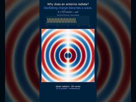
Electric Dipole | the field two opposite charges weave #Shorts