NovaSolver›Bernoulli's Equation — Fluid Flow Visualizer Back
Fluid Dynamics
Bernoulli's Equation — Fluid Flow Visualizer
Visualize pressure, velocity, and hydraulic head in a pipe system in real time. Experience the core of fluid mechanics through Venturi tubes, Pitot tubes, and airfoil lift via animated charts.
Venturi Tube (water)Venturi Tube (air)Horizontal Pipe to Downward FlowHigh-Speed Throat
Bernoulli's Theorem
$\frac{P}{\rho g} + \frac{v^2}{2g} + z = H = \text{const}$
$P_1 + \frac{1}{2}\rho v_1^2 + \rho g z_1 = P_2 + \frac{1}{2}\rho v_2^2 + \rho g z_2$
Continuity equation: $A_1 v_1 = A_2 v_2$
Results
8.00
Throat Velocity V₂ (m/s)
101.3
Inlet Pressure P₁ (kPa)
69.3
Throat Pressure P₂ (kPa)
15.7
Flow Rate Q (L/s)
Pipe Cross-Section
Hydraulic Head Diagram
P-V Distribution
Pipe
Head
💬 Ask the Professor
🙋
I understand that velocity increases and pressure drops when a pipe narrows, but intuitively, why does higher speed mean lower pressure?
🎓
It is an energy balance. The fluid's total energy is the sum of pressure energy, kinetic energy, and potential energy. When velocity increases, kinetic energy increases, so pressure energy decreases. The stronger jet you get by partly covering a faucet with your thumb follows the same velocity-up, pressure-down relationship.
🙋
How does a Venturi tube measure flow rate?
🎓
You measure only the pressure difference ΔP between the wide section and the throat. The continuity equation gives V₂=V₁·(A₁/A₂), and Bernoulli's equation relates that velocity ratio to ΔP. From there, Q=A₁V₁ gives the flow rate. Because there are no moving parts, Venturi meters are robust and still used in water and petroleum pipelines.
🙋
What happens if the pressure becomes very low? The simulator shows the throat pressure dropping.
🎓
That is cavitation. When pressure falls below the liquid's vapor pressure, the liquid locally boils and vapor bubbles form. When those bubbles collapse in a higher-pressure region, they can generate shock waves that erode pumps and hydrofoils. In CFD, checking that the minimum pressure stays above the liquid vapor pressure is essential.
🙋
I have heard aircraft wings can be explained by Bernoulli's equation, but also that this is not strictly correct. Which is true?
🎓
Both contain some truth. Bernoulli's equation can explain the qualitative idea that faster flow over the upper surface corresponds to lower pressure and lift. However, the common story that upper and lower streams must meet at the trailing edge at the same time is false. A rigorous explanation uses circulation and the Kutta-Joukowski theorem, L=ρVΓ, which is also the framework behind many CFD interpretations.
Frequently Asked Questions
When the cross-sectional area is reduced, the flow velocity increases according to the continuity equation, and the pressure decreases according to Bernoulli's theorem. Conversely, when the cross-sectional area is increased, the flow velocity decreases and the pressure recovers. This can be observed in real time through bar graphs and streamline colors on the screen.
The Pitot tube utilizes the difference between total pressure (stagnation pressure) and static pressure. Total pressure is the pressure at the point where the flow is stopped, while static pressure is the surrounding pressure. By substituting this differential pressure into Bernoulli's theorem, the flow velocity can be calculated. In the simulator, this is displayed numerically and graphically.
Increasing the angle of attack further increases the flow velocity on the upper surface of the wing, widening the velocity difference between the upper and lower surfaces. This increases the lift coefficient, but beyond a certain angle, the flow separates and stall occurs. The simulator allows visual confirmation of changes in lift and disturbances in streamlines.
No. This simulator is based on an ideal fluid model of inviscid, incompressible, steady flow, and does not account for energy losses due to pipe friction or viscosity. Therefore, the numerical values do not perfectly match real phenomena, but it is suitable for understanding the essence of Bernoulli's theorem.
What is Fluid Bernoulli?
Fluid Bernoulli is a fundamental topic in engineering and applied physics. This interactive simulator lets you explore the key behaviors and relationships by directly manipulating parameters and observing real-time results.
By combining numerical computation with visual feedback, the simulator bridges the gap between abstract theory and physical intuition — making it an effective learning tool for students and a rapid-verification tool for practicing engineers.
Physical Model & Key Equations
The simulator is based on the governing equations behind Bernoulli's Equation — Fluid Flow Visualizer. Understanding these equations is key to interpreting the results correctly.
Each parameter in the equations corresponds to a slider in the control panel. Moving a slider changes the equation's solution in real time, helping you build a direct connection between mathematical expressions and physical behavior.
Real-World Applications
Engineering Design: The concepts behind Bernoulli's Equation — Fluid Flow Visualizer are applied across mechanical, structural, electrical, and fluid engineering disciplines. This tool provides a quick way to estimate design parameters and sensitivity before committing to full CAE analysis.
Education & Research: Widely used in engineering curricula to connect theory with numerical computation. Also serves as a first-pass validation tool in research settings.
CAE Workflow Integration: Before running finite element (FEM) or computational fluid dynamics (CFD) simulations, engineers use simplified models like this to establish physical scale, identify dominant parameters, and define realistic boundary conditions.
Common Misconceptions and Points of Caution
Model assumptions: The mathematical model used here relies on simplifying assumptions such as linearity, homogeneity, and isotropy. Always verify that your real system satisfies these assumptions before applying results directly to design decisions.
Units and scale: Many calculation errors arise from unit conversion mistakes or order-of-magnitude errors. Pay close attention to the units shown next to each parameter input.
Validating results: Always sanity-check simulator output against physical intuition or hand calculations. If a result seems unexpected, review your input parameters or verify with an independent method.
Enter upstream pipe diameter (d1) in millimeters and downstream diameter (d2) to define the flow restriction geometry
Input upstream velocity (v1) in m/s and elevation (z1) in meters relative to your reference datum
The simulator calculates downstream velocity (v2) using continuity equation A1·v1 = A2·v2, then applies Bernoulli's equation to solve for pressure head changes: (P1/ρg) + (v1²/2g) + z1 = (P2/ρg) + (v2²/2g) + z2
Worked Example
Water flows through a venturi meter with d1=50mm, d2=25mm (area ratio 4:1), v1=2 m/s, z1=0m. Continuity gives v2=8 m/s. Using Bernoulli with ρ=1000 kg/m³ and g=9.81 m/s²: pressure head drop = (v2²−v1²)/(2g) = (64−4)/(19.62) ≈ 3.06m water column. At d2, static pressure decreases significantly due to velocity increase, enabling flow measurement in industrial pipelines.
Practical Notes
Assume frictionless flow—real pipe losses require adding head loss terms (Darcy-Weisbach) for accuracy in systems with long runs or high roughness
Verify z1 and z2 reference elevations consistently; even 0.5m elevation change affects pressure head by ~5 kPa in water applications
Watch for cavitation risk when downstream pressure drops below 2.4 kPa absolute in centrifugal pumps or venturi sections
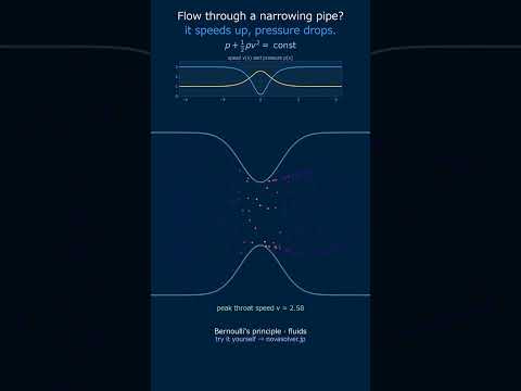
🎬 Watch it in motion
Flow speeds up in narrow spots — Bernoulli's principle #Shorts