Contact Mechanics in MBD
Theory and Physics
MBD Contact
Professor, how is contact in MBD different from contact in FEM?
FEM contact is surface contact between deformable bodies. MBD contact is contact between rigid bodies (collision, meshing, etc.). The computation is lighter but does not include deformation.
MBD Contact Force Model
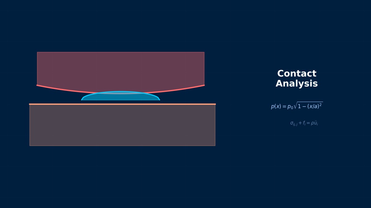
The Hertz contact model is fundamental:
$\delta$: penetration depth, $K$: Hertz stiffness, $D$: damping. For sphere-sphere, sphere-plane contact.
Summary
Hertz contact theory originates from a paper submitted by the 24-year-old Hertz in 1882
The classical theory of elastic contact, "Hertz contact," originates from a paper submitted by Heinrich Hertz (then 24 years old) in 1882 to the "Journal für die reine und angewandte Mathematik." Hertz is said to have conceived the mathematical model for contact area while observing interference fringes of light through glass lenses and completed it in two weeks. This theory is directly used in the design of rolling bearings, gears, and railway wheels today, and continues to be active as the fundamental equation for contact models in multibody systems for over 140 years.
Physical Meaning of Each Term
- Inertia term (mass term): $\rho \ddot{u}$, i.e., "mass × acceleration". Have you ever experienced being thrown forward when slamming on the brakes? That "feeling of being carried away" is precisely the inertial force. Heavier objects are harder to set in motion and harder to stop once moving. Buildings shake during earthquakes because the ground moves suddenly while the building's mass "gets left behind." In static analysis, this term is set to zero, which is the assumption that "acceleration can be ignored because the force is applied slowly." It absolutely cannot be omitted in impact loads or vibration problems.
- Stiffness term (elastic restoring force): $Ku$ or $\nabla \cdot \sigma$. When you stretch a spring, you feel a "force trying to return it," right? That is Hooke's law $F=kx$, and it's the essence of the stiffness term. Now a question—if you pull an iron rod and a rubber band with the same force, which stretches more? Obviously, the rubber band. This "resistance to stretching" is the Young's modulus $E$, which determines stiffness. A common misconception: "high stiffness = strong" is incorrect. Stiffness is "resistance to deformation," strength is "resistance to failure"—they are different concepts.
- External force term (load term): Body forces $f_b$ (gravity, etc.) and surface forces $f_s$ (pressure, contact force, etc.). Think of it this way—the weight of a truck on a bridge is a "force acting on the entire interior" (body force), while the force of the tires pushing on the road surface is a "force acting only on the surface" (surface force). Wind pressure, water pressure, bolt tightening force... all are external forces. A common mistake here: getting the load direction wrong. Intending "tension" but it becomes "compression"—it sounds like a joke, but it actually happens when coordinate systems are rotated in 3D space.
- Damping term: Rayleigh damping $C\dot{u} = (\alpha M + \beta K)\dot{u}$. Try plucking a guitar string. Does the sound continue forever? No, it gradually fades away. That's because the vibration energy is converted to heat by air resistance and internal friction in the string. Car shock absorbers work on the same principle—they intentionally absorb vibration energy to improve ride comfort. What if damping were zero? Buildings would continue shaking forever after an earthquake. Since that doesn't happen in reality, setting appropriate damping is crucial.
Assumptions and Applicability Limits
- Continuum assumption: Treats material as a continuous medium, ignoring microscopic heterogeneity.
- Small deformation assumption (for linear analysis): Deformation is sufficiently small compared to initial dimensions, and the stress-strain relationship is linear.
- Isotropic material (unless otherwise specified): Material properties are independent of direction (anisotropic materials require separate tensor definitions).
- Quasi-static assumption (for static analysis): Ignores inertial and damping forces, considering only the balance between external and internal forces.
- Non-applicable cases: For large deformation/large rotation problems, geometric nonlinearity is required. For nonlinear material behavior like plasticity or creep, constitutive law extensions are needed.
Dimensional Analysis and Unit Systems
| Variable | SI Unit | Notes / Conversion Memo |
|---|---|---|
| Displacement $u$ | m (meter) | When inputting in mm, unify load and elastic modulus to MPa/N system. |
| Stress $\sigma$ | Pa (Pascal) = N/m² | MPa = 10⁶ Pa. Be careful of unit system inconsistency when comparing with yield stress. |
| Strain $\varepsilon$ | Dimensionless (m/m) | Note the distinction between engineering strain and logarithmic strain (for large deformation). |
| Elastic modulus $E$ | Pa | Steel: ~210 GPa, Aluminum: ~70 GPa. Note temperature dependence. |
| Density $\rho$ | kg/m³ | In mm system: tonne/mm³ (= 10⁻⁹ tonne/mm³ for steel). |
| Force $F$ | N (Newton) | Unify as N in mm system, N in m system. |
Numerical Methods and Implementation
MBD Contact Implementation
Summary
The choice between penalty method and constraint stabilization method determines accuracy
The main methods for multibody contact analysis are divided into two categories: the penalty method (generates reaction force proportional to penetration) and the Baumgarte constraint stabilization method. If the penalty stiffness is too high, numerical integration becomes unstable; if too low, unrealistic penetration occurs. MSC Adams, since its 2010 version, implemented an algorithm that automatically estimates the default contact stiffness as "material Young's modulus × square root of contact area," significantly reducing user calculation divergence troubles caused by setting failures.
Linear Elements (1st-order elements)
Linear interpolation between nodes. Low computational cost but low stress accuracy. Beware of shear locking (mitigated by reduced integration or B-bar method).
Quadratic Elements (with mid-side nodes)
Can represent curved deformation. Stress accuracy improves significantly, but degrees of freedom increase by about 2-3 times. Recommended: when stress evaluation is important.
Full integration vs Reduced integration
Full integration: Risk of over-constraint (locking). Reduced integration: Risk of hourglass modes (zero-energy modes). Choose appropriately for the situation.
Adaptive Mesh
Automatic refinement based on error indicators (e.g., ZZ estimator). Efficiently improves accuracy in stress concentration areas. Includes h-method (element subdivision) and p-method (order increase).
Newton-Raphson Method
Standard method for nonlinear analysis. Updates the tangent stiffness matrix every iteration. Provides quadratic convergence within the convergence radius but has high computational cost.
Modified Newton-Raphson Method
Updates the tangent stiffness matrix using the initial value or every few iterations. Cost per iteration is low, but convergence speed is linear.
Convergence Criteria
Force residual norm: $||R|| / ||F_{ext}|| < \epsilon$ (typically $\epsilon = 10^{-3}$ to $10^{-6}$). Displacement increment norm: $||\Delta u|| / ||u|| < \epsilon$. Energy norm: $\Delta u \cdot R < \epsilon$.
Load Increment Method
Applies the total load not all at once but in small increments. The arc-length method (Riks method) can track beyond limit points on the load-displacement curve.
Analogy: Direct Method vs Iterative Method
The direct method is like "solving simultaneous equations accurately with pen and paper"—reliable but takes too long for large-scale problems. The iterative method is like "repeatedly guessing to approach the correct answer"—the initial answer is rough, but accuracy improves with each iteration. It's the same principle as looking up a word in a dictionary: it's more efficient to estimate where to open it and adjust forward/backward (iterative method) than to search sequentially from the first page (direct method).
Relationship Between Mesh Order and Accuracy
1st-order elements are like "approximating a curve with a ruler"—represented by straight line segments, so accuracy is limited. 2nd-order elements are like "flexible curves"—can represent curved changes, dramatically improving accuracy even at the same mesh density. However, computational cost per element increases, so judgment should be based on total cost-effectiveness.
Practical Guide
MBD Contact in Practice
Power transmission in gear trains, chain motion, ball bearing dynamics.
Practical Checklist
Cam-follower contact is the most frequently analyzed case in MBD
Cam-follower contact in engine valve mechanisms is one of the most typical practical applications of multibody contact analysis. Honda's inline 4-cylinder engine (2.0L) used MBD contact analysis to predict cam-follower bouncing (contact separation) at high RPMs (above 6500 rpm), and the history of optimizing the valve spring design over two generations is documented in the Honda R&D Technical Review (2004).
Analogy: Analysis Flow
The analysis flow is actually very similar to cooking. First, you buy the ingredients (prepare the CAD model), do the prep work (mesh generation), apply heat (solver execution), and finally plate it (visualization in post-processing). Here's an important question—which step in cooking is most prone to failure? Actually, it's the "prep work." If the mesh quality is poor, the results will be a mess no matter how excellent the solver is.
Pitfalls Beginners Often Fall Into
Are you checking mesh convergence? Do you think "the calculation ran = the results are correct"? This is actually the most common trap for CAE beginners. The solver will always return "some answer" for the given mesh. But if the mesh is too coarse, that answer can be far from reality. Confirm that results stabilize with at least three levels of mesh density—neglecting this leads to the dangerous assumption that "the computer gave the answer, so it must be correct."
Thinking About Boundary Conditions
Setting boundary conditions is like "writing the problem statement" for an exam. If the problem statement is wrong? No matter how accurately you calculate, the answer will be wrong. "Is this surface really fully fixed?" "Is this load really uniformly distributed?"—Correctly modeling the real-world constraint conditions is actually the most important step in the entire analysis.
Software Comparison
MBD Contact Tools
RecurDyn holds a top global market share in gear/chain contact analysis
RecurDyn by Korea's FunctionBay specializes in analyzing gear trains, chain drives, and belt mechanisms involving numerous contacting bodies with its fast algorithm (MFBD: Multi-Flexible Body Dynamics), forming a duopoly with MSC Adams in the manufacturing-oriented contact MBD market. The Hyundai Motor Group has adopted RecurDyn for contact analysis of engine accessory belts and automatic transmissions, and has published comparative data showing it is 10 times faster than Adams for chain multi-contact problems.
The Three Most Important Questions for Selection
- "What are you solving?": Does it support the physical models/element types needed for contact mechanics in MBD? For example, in fluids, the presence of LES support; in structures, the capability for contact/large deformation makes the difference.
- "Who will use it?": For beginner teams, tools with rich GUIs are suitable; for experienced users, flexible script-driven tools are better. Similar to the difference between automatic transmission cars (GUI) and manual transmission cars (script).
- "How far will it expand?": Selection considering future analysis scale expansion (HPC support), expansion to other departments, and integration with other tools leads to long-term cost reduction.
Advanced Technology
Advanced MBD Contact
Real-time MBD contact is the key to autonomous vehicle simulator development
Real-time multibody dynamics with contact is an essential technology for driving simulators used in autonomous vehicle development. Mechanical Simulation Corporation's CarSim, used by Toyota and GM, achieves real-time calculation of tire-road contact (Pacejka model) and suspension dynamics at 1 kHz. The contact force calculation algorithm is optimized for x86 multi-core CPUs, enabling high-fidelity vehicle dynamics simulation with a time step of 1 ms.
Future Outlook
- AI/ML-assisted contact parameter identification: Automatically tuning contact stiffness/damping from experimental data.
- Digital twin integration: Real-time MBD contact models synchronized with physical sensors.
- Quantum-inspired optimization: For topology optimization of contact surfaces.
Related Topics
なった
詳しく
報告