UAV Aerodynamic Design
Theory and Physics
Overview
Professor, how is the aerodynamic design of drones and UAVs different from that of manned aircraft?
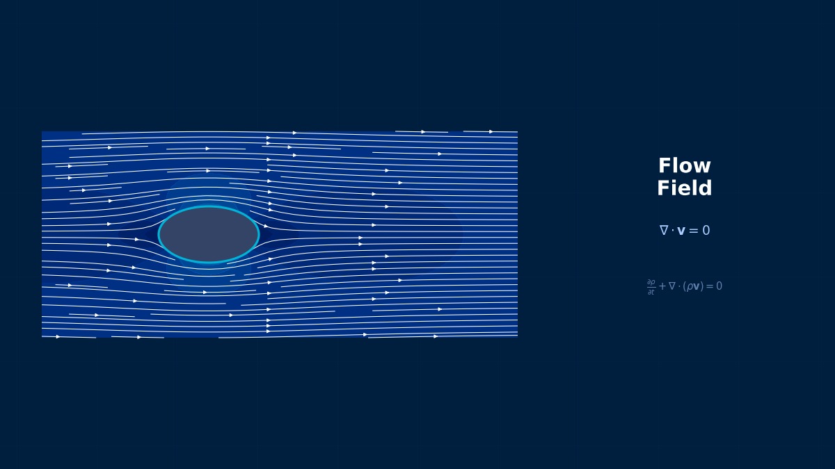
The biggest difference is the Reynolds number. While manned aircraft fly at $Re \sim 10^7$, small UAVs operate in the low Reynolds number regime of $Re \sim 10^4$--$10^6$. In this regime, laminar separation bubbles and transition phenomena dominate performance.
Key points to consider in UAV aerodynamic design:
- Selection of low-Re airfoils (e.g., Eppler, Selig/Donovan airfoils)
- Propeller-airframe interference
- Multi-rotor mutual interference
- Gust response (significant impact due to small airframe size)
Low Reynolds Number Aerodynamics
Airfoil characteristics in the low-Re regime are qualitatively different from those in the high-Re regime.
| Re Range | Flow Characteristics | Applicable UAVs |
|---|---|---|
| $10^4$--$10^5$ | Laminar separation bubble dominant, transition unstable | Micro UAVs, insect-like |
| $10^5$--$10^6$ | Transition location determines performance | Small fixed-wing UAVs |
| $10^6$--$10^7$ | Similar to manned aircraft | Large MALE/HALE UAVs |
What is a laminar separation bubble?
At low Re, the boundary layer remains laminar and separates due to an adverse pressure gradient. The separated free shear layer transitions to turbulence and reattaches. This region of separation-transition-reattachment is the "laminar separation bubble." The size and location of the bubble significantly affect lift and drag.
So the maximum lift coefficient decreases at low Re.
Propeller Aerodynamics
Propeller aerodynamics for UAVs is also an important subject for CFD.
Propeller thrust coefficient and efficiency:
Where $T$ is thrust, $n$ is rotational speed [rps], $D$ is propeller diameter, $J = V_\infty/(nD)$ is the advance ratio, and $C_P$ is the power coefficient.
For multi-rotors, how much does interference between propellers affect performance?
When the wake (downwash) of adjacent propellers interferes, hovering efficiency can decrease by 5--15%. Interference becomes significant when the propeller spacing is less than 1.5 times the diameter. Evaluating this interference effect with CFD is essential for efficient airframe design.
The World of Ultra-Low Reynolds Numbers – Flying Under the Same Conditions as Insects
Small UAV propellers, with diameters of 10-20 cm, operate in the "ultra-low Re regime" of Re=10,000–100,000. This is a challenging region where airfoil performance changes dramatically, and laminar separation bubbles frequently occur. Interestingly, insects fly in the same regime. Research on the flight mechanisms of bees and butterflies is directly applied to UAV airfoil design. Biomimetic designs learned from living creatures are quietly incorporated into modern commercial drones.
Physical Meaning of Each Term
- Temporal Term $\partial(\rho\phi)/\partial t$: Imagine turning on a faucet. At first, water comes out spluttering and unstable, but after a while, the flow becomes steady, right? This "during the change" is described by the temporal term. The pulsation of blood flow from a heartbeat, or the flow fluctuation each time an engine valve opens and closes—all are unsteady phenomena. So what is steady-state analysis? It looks only at "after sufficient time has passed and the flow has settled down"—meaning this term is set to zero. Since computational cost is significantly reduced, starting with a steady-state solution is a basic CFD strategy.
- Convection Term $\nabla \cdot (\rho \mathbf{u} \phi)$: What happens if you drop a leaf into a river? It gets carried downstream by the flow, right? This is "convection"—the effect where fluid motion transports things. Warm air from a heater reaching the far corner of a room is also due to air, the "carrier," transporting heat via convection. Here's the interesting part—this term contains "velocity × velocity," making it nonlinear. That is, as the flow becomes faster, this term rapidly strengthens, making control difficult. This is the root cause of turbulence. A common misconception: "Convection and conduction are similar" → They are completely different! Convection is carried by flow, conduction is transmitted by molecules. There's an order of magnitude difference in efficiency.
- Diffusion Term $\nabla \cdot (\Gamma \nabla \phi)$: Have you ever put milk in coffee and left it? Even without stirring, after a while it naturally mixes, right? That's molecular diffusion. Now a question—honey or water, which flows more easily? Obviously water, right? Honey has high viscosity ($\mu$), so it flows poorly. Higher viscosity strengthens the diffusion term, making the fluid move "sluggishly." In low Reynolds number flows (slow, viscous), diffusion dominates. Conversely, in high-Re flows, convection overwhelms and diffusion plays a minor role.
- Pressure Term $-\nabla p$: When you push the plunger of a syringe, liquid shoots out forcefully from the needle tip, right? Why? Because the piston side is high pressure, the needle tip is low pressure—this pressure difference provides the force that pushes the fluid. Dam discharge works on the same principle. On a weather map, where isobars are tightly packed? That's right, strong winds blow. "Flow arises where there is a pressure difference"—this is the physical meaning of the pressure term in the Navier-Stokes equations. A point of confusion here: "Pressure" in CFD is often gauge pressure, not absolute pressure. If results become strange when switching to compressible analysis, it might be due to mixing up absolute/gauge pressure.
- Source Term $S_\phi$: Heated air rises—why? Because it becomes lighter (lower density) than its surroundings, so buoyancy pushes it upward. This buoyancy is added to the equation as a source term. Other examples: chemical reaction heat from a gas stove flame, Lorentz force acting on molten metal in a factory's electromagnetic pump... These are all actions that "inject energy or force into the fluid from the outside," expressed by the source term. What happens if you forget the source term? In natural convection analysis, forgetting buoyancy means the fluid doesn't move at all—a physically impossible result where warm air doesn't rise in a heated room in winter.
Assumptions and Applicability Limits
- Continuum assumption: Valid for Knudsen number Kn < 0.01 (molecular mean free path ≪ characteristic length)
- Newtonian fluid assumption: Linear relationship between shear stress and strain rate (non-Newtonian fluids require viscosity models)
- Incompressibility assumption (for Ma < 0.3): Density treated as constant. For Mach numbers above 0.3, compressibility effects must be considered.
- Boussinesq approximation (Natural Convection): Density variation considered only in the buoyancy term; constant density used in other terms.
- Non-applicable cases: Rarefied gases (Kn > 0.1), supersonic/hypersonic flow (shock capturing required), free surface flow (requires VOF/Level Set, etc.)
Dimensional Analysis and Unit Systems
| Variable | SI Unit | Notes / Conversion Memo |
|---|---|---|
| Velocity $u$ | m/s | When converting from volumetric flow rate for inlet conditions, pay attention to cross-sectional area units. |
| Pressure $p$ | Pa | Distinguish between gauge and absolute pressure. Use absolute pressure for compressible analysis. |
| Density $\rho$ | kg/m³ | Air: approx. 1.225 kg/m³ @20°C, Water: approx. 998 kg/m³ @20°C |
| Viscosity coefficient $\mu$ | Pa·s | Be careful not to confuse with kinematic viscosity coefficient $\nu = \mu/\rho$ [m²/s] |
| Reynolds number $Re$ | Dimensionless | $Re = \rho u L / \mu$. Indicator for laminar/turbulent transition. |
| CFL number | Dimensionless | $CFL = u \Delta t / \Delta x$. Directly related to time step stability. |
Numerical Methods and Implementation
Numerical Methods for Low-Re Airfoils
What's important when solving low Reynolds number airfoils with CFD?
The choice of transition model is most important. RANS models assuming fully turbulent flow cannot reproduce low-Re airfoil characteristics at all.
| Model | Characteristics | Suitability for Low-Re Airfoils |
|---|---|---|
| SST k-omega (Fully Turbulent) | No transition | Unsuitable. Overestimates $C_D$, inaccurate $C_{L,max}$ |
| $\gamma$-$Re_\theta$ Transition Model | RANS transition prediction | Good. Reproduces laminar separation bubbles. |
| k-kl-omega | 3-equation transition model | Good. Suitable for low Re. |
| LES | Directly resolves large-scale eddies | Highest accuracy but high cost. |
| XFOIL (Panel Method + BL) | 2D only. Fast. | Optimal for initial design. |
XFOIL is still widely used today, isn't it?
XFOIL, developed by Mark Drela, is a standard tool for low-Re airfoil design. It combines a panel method with a boundary layer coupling method, completing analyses including transition and laminar separation bubbles in seconds. For initial screening, XFOIL is more efficient than CFD.
Propeller CFD
How do you analyze propellers?
There are three main methods.
| Method | Modeling | Accuracy | Cost |
|---|---|---|---|
| BEM (Blade Element Momentum) | 1D theory | Medium | Very Low |
| Virtual Disk (Actuator Disk) | Represents propeller with body forces | Medium | Low |
| Full Blade Analysis | Directly solves blade geometry with 3D CFD | High | High |
- BEM: Used for parametric studies of thrust/efficiency in initial design.
- Virtual Disk: Rough estimation of propeller-airframe interference. Models available in Fluent/STAR-CCM+.
- Full Blade: Rotates blades using sliding mesh or overset mesh. Requires unsteady analysis.
What's the principle behind the virtual disk model?
A thin disk region is set at the propeller location, and body forces equivalent to the thrust and torque calculated by BEM theory are applied. Since the blade shape does not need to be resolved by the mesh, it is efficient for evaluating propeller-airframe interference.
Multi-Rotor CFD
CFD strategy for multi-rotors (e.g., quadcopters):
- Hovering: Steady-state analysis of each rotor using virtual disk or MRF.
- Forward Flight: Requires unsteady analysis. Captures periodic rotor fluctuations.
- Rotor Interference: Downwash from upper rotors affects lower ones (in coaxial rotor configurations).
- Mesh Scale: 100-300 million cells for full-blade LES of a 4-rotor system.
Setting the rotation direction for each rotor in STAR-CCM+'s Rigid Body Motion is crucial. Adjacent rotors should rotate in opposite directions to cancel out reaction torque. Getting the rotation direction wrong will generate a yaw moment.
The Secret CFD Verification Story of the Mars Helicopter Ingenuity
NASA's Mars helicopter Ingenuity flew in the ultra-low density atmosphere of Mars (approx. 1/100th of Earth's, 0.02 kg/m³). Wind tunnel experiments on Earth were extremely difficult to replicate "Martian atmospheric pressure," making CFD the primary design tool. The particular challenge was the combination of low Re × high Mach number (blade tip speed exceeding 70% of the speed of sound), a regime outside the applicability of typical aerodynamic CFD. The design process, which combined detailed CFD including compressibility effects with partial vacuum chamber experiments, serves as a highly instructive case study in CFD application.
Upwind Scheme
First-order upwind: Large numerical diffusion but stable. Second-order upwind: Improved accuracy but risk of oscillations. Essential for high Reynolds number flows.
Central Differencing
Second-order accurate, but numerical oscillations occur for Peclet number > 2. Suitable for low Reynolds number diffusion-dominated flows.
TVD Schemes (MUSCL, QUICK, etc.)
Maintain high accuracy while suppressing numerical oscillations via limiter functions. Effective for capturing shocks and steep gradients.
Finite Volume Method vs Finite Element Method
FVM: Naturally satisfies conservation laws. Mainstream in CFD. FEM: Advantageous for complex shapes and multi-physics. Mesh-free methods like SPH are also developing.
CFL Condition (Courant Number)
Explicit methods: CFL ≤ 1 is the stability condition. Implicit methods: Stable even for CFL > 1, but affects accuracy and iteration count. LES: CFL ≈ 1 recommended. Physical meaning: Information should not travel more than one cell per time step.
Residual Monitoring
Convergence is judged when residuals for Continuity Equation, momentum, and energy drop by 3-4 orders of magnitude. The mass conservation residual is particularly important.
Relaxation Factor
Typical initial values: Pressure: 0.2–0.3, Velocity: 0.5–0.7. Reduce the factor if diverging. Increase after convergence to accelerate.
Internal Iterations for Unsteady Calculations
Iterate within each time step until a steady solution converges. Internal iteration count: 5–20 iterations is a guideline. If residuals fluctuate between time steps, review the time step size.
Analogy for the SIMPLE Method
The SIMPLE method is an "alternating adjustment" technique. First, velocity is tentatively determined (predictor step), then pressure is corrected so that mass conservation is satisfied with that velocity (corrector step), and velocity is revised using the corrected pressure—this back-and-forth is repeated to approach the correct solution. It resembles two people leveling a shelf: one adjusts the height, the other balances it, and they repeat this alternately.
Analogy for the Upwind Scheme
The upwind scheme is a method that "stands in the river flow and prioritizes upstream information." A person in the river cannot tell the source of the water by looking downstream—it reflects the physics that upstream information determines downstream conditions. Although first-order accurate, it is highly stable because it correctly captures flow direction.
Practical Guide
Analysis Workflow
Please teach me a typical CFD workflow for UAV aerodynamic design.
Related Topics
なった
詳しく
報告