Linear Buckling (Eigenvalue Buckling) Analysis
Linear Buckling (Eigenvalue Buckling) Analysis: Theoretical Foundations
Overview
Professor, are "linear buckling analysis" and "eigenvalue buckling analysis" the same thing?
They are the same. In the context of FEM, "linear buckling analysis," "eigenvalue buckling analysis," and "linearized pre-buckling analysis" all refer to the same method. It is a technique that creates a geometric stiffness matrix from the stress state of the reference configuration, solves an eigenvalue problem, and obtains the buckling load factor.
It's the $([K] + \lambda [K_\sigma])\{\phi\} = \{0\}$ we learned in the Euler buckling section, right? Does that mean applying it to general structures?
Exactly. Euler buckling was limited to the specific structure of a "column," but eigenvalue buckling analysis is a general method applicable to plates, shells, frames, and even their combined structures.
Mathematical Structure of Eigenvalue Buckling Analysis
Could you explain the general formula in a bit more detail?
It's a two-step procedure.
Step 1: Perform a static analysis under the reference load $\{F_{ref}\}$ to obtain the stress distribution $\{\sigma_{ref}\}$:
Step 2: Construct the geometric stiffness matrix $[K_\sigma]$ from the obtained stress and solve the eigenvalue problem:
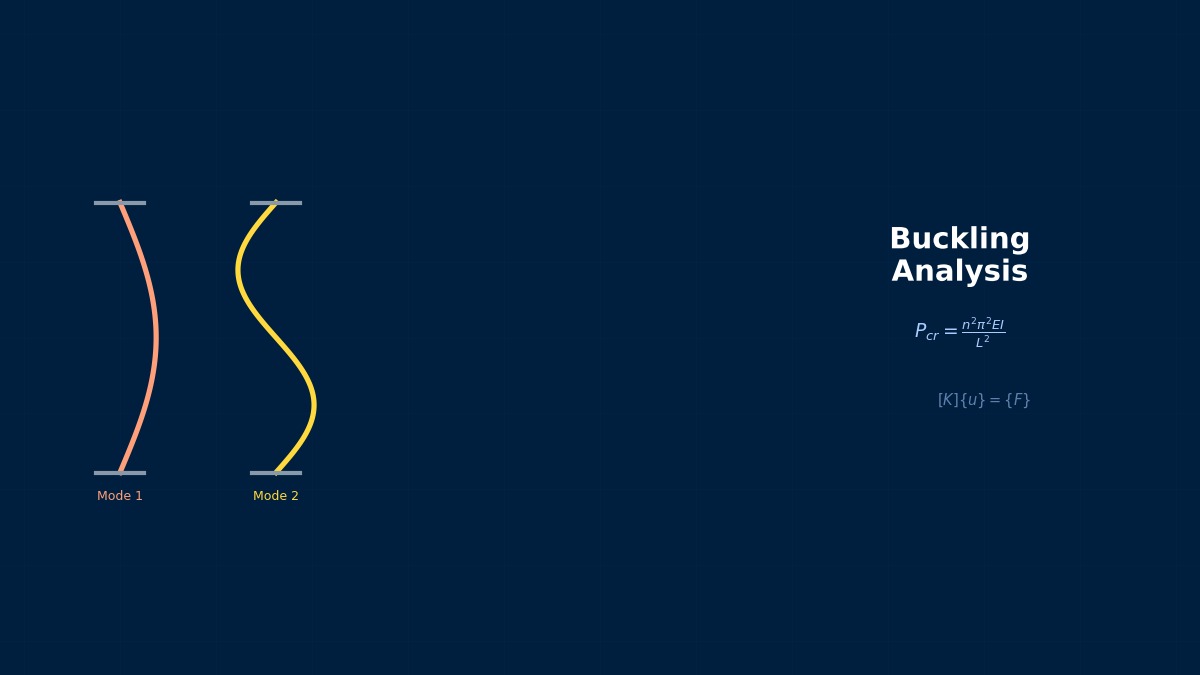
$\lambda_i$ is the buckling load factor, and $\{\phi_i\}$ is the mode shape. If $\lambda_1 = 3.5$, it buckles at 3.5 times the reference load.
Correct. The important point here is that the static analysis in Step 1 is a linear static analysis. That means it does not consider large deformation effects. Under the assumption that stress increases proportionally with load, it predicts "when instability occurs."
That's why it's called "linear" buckling analysis.
Precisely. This "assumption of linearity" is the essential limitation of eigenvalue buckling analysis and simultaneously the source of its computational speed.
Why It Becomes an Eigenvalue Problem
First of all, why can buckling be formulated as an eigenvalue problem?
That's a fundamental question. Buckling is a phenomenon where "the deformation suddenly transitions from a state that was constant despite increasing load to a different deformation pattern." Mathematically, it is viewed as a bifurcation of the equilibrium path.
When scaling the load as $\lambda \{F_{ref}\}$, the overall stiffness becomes $[K_0] + \lambda [K_\sigma]$. Here, $[K_\sigma]$ is the geometric stiffness for the reference stress, so it scales proportionally with $\lambda$. The point where this overall stiffness becomes singular (det = 0) is the bifurcation point, and that $\lambda$ is the buckling load factor.
Finding the $\lambda$ where the determinant of $[K_0] + \lambda [K_\sigma]$ becomes zero... that takes the form of an eigenvalue problem!
Yes. It has exactly the same mathematical structure as vibration analysis $([K] - \omega^2 [M])\{\phi\} = \{0\}$. In vibration, the mass matrix $[M]$ is in that position; in buckling, the geometric stiffness matrix $[K_\sigma]$ is there.
Physical Meaning of the Geometric Stiffness Matrix
Could you explain the physical meaning of $[K_\sigma]$ a bit more?
$[K_\sigma]$ represents "how much work the current stress state does against a small displacement perturbation." If you deflect a beam element under compressive stress slightly sideways, the compressive force does work in the direction that increases the deflection. This acts as a negative stiffness.
To be specific, for a beam element under axial force $N$, when a small lateral deflection $\delta v$ occurs, the axial force does additional work of $N \cdot (\delta v')^2 / 2$. This "additional work due to stress" is what is matrix-formulated as $[K_\sigma]$.
Under compression ($N < 0$) stiffness decreases, under tension ($N > 0$) stiffness increases. That's why tensile members don't buckle, right?
That intuition is correct. However, there is a caveat. For example, even tensile members like prestressed cables can experience lateral buckling (a phenomenon essentially close to the vibration mode of a tensile member). Basically, you can understand it as "the part dominated by compressive stress is the starting point of buckling."
Premises and Limitations of Linear Buckling Analysis
Under what conditions does linear buckling analysis give the "correct answer"?
It is highly reliable when the following premises are met:
1. Pre-buckling deformation is small — The shape remains virtually unchanged.
2. Material is within the elastic range — No yielding at the buckling point.
3. Loads are proportional — All loads increase or decrease at the same ratio.
4. Initial imperfections are small — Deviations from the ideal shape are negligible.
What if these are not met?
The result of eigenvalue buckling analysis becomes an upper bound (unconservative estimate). That is, the actual collapse load is lower than the eigenvalue buckling load. How much lower specifically depends on the structure type:
| Structure Type | Reliability of Eigenvalue Buckling | Actual Collapse Load / Eigenvalue Buckling Load |
|---|---|---|
| Column (global buckling) | High | 0.85 ~ 1.0 |
| Flat Plate (in-plane compression) | Relatively High | 0.7 ~ 0.95 |
| Cylindrical Shell (axial compression) | Very Low | 0.2 ~ 0.5 |
| Stiffened Panel | Medium | 0.5 ~ 0.9 |
Cylindrical shells can drop to as low as one-fifth...?
That's why for buckling design of cylindrical shells, eigenvalue analysis alone is insufficient, and nonlinear analysis incorporating initial imperfections is essential. On the other hand, global buckling of columns can be estimated quite well with eigenvalue analysis. In practice, it is extremely important to understand the "reliability of eigenvalue analysis" according to the structure type.
Summary
To summarize the theory of eigenvalue buckling analysis...
It's important to recognize that eigenvalue buckling analysis is a "screening tool," not the "final answer."
Exactly. It is an optimal method for quickly finding "where is dangerous" in the early stages of design. However, don't forget that whether you can give a design OK based on it alone depends on the structure's imperfection sensitivity.
Origins of Eigenvalue Buckling Analysis and Hertz Contact
Eigenvalue buckling analysis (linear buckling analysis) was already formulated as a matrix eigenvalue problem in the 1950s-60s, before the FEM era. Shortly after Turner and Clough (1960) applied FEM to structural analysis, Martin (1965) introduced the geometric stiffness matrix, leading to the birth of linear buckling FEM. NASTRAN (1968) was the first to commercially implement this.
Computational Methods for Linear Buckling (Eigenvalue Buckling) Analysis
Internal Operation of Eigenvalue Solvers
What algorithm specifically solves $([K_0] + \lambda [K_\sigma])\{\phi\} = \{0\}$ and how does it work?
Eigenvalue problems in structural analysis are typically generalized eigenvalue problems. For buckling, when transformed to standard form:
$[K_0]$ is positive definite symmetric (if properly constrained), $[K_\sigma]$ is symmetric but indefinite. There are several efficient algorithms that utilize this structure.
Lanczos Method
I've heard the Lanczos method is standard in practice, why is that?
The Lanczos method is the most widely used eigenvalue solver for structural problems because of its combination of efficiency and scalability. It is a subspace iteration method that projects the full problem onto a small Krylov subspace, working with sparse matrix–vector products rather than explicit matrix factorization.
Key advantages:
1. Memory efficient — Does not require storing the factorization, only sparse matrix storage
2. Fast convergence — Excellent at finding the first few eigenvalues/eigenvectors, which is usually all we need
3. Robust against ill-conditioning — Works well even when the eigenvalues are clustered
4. Parallelizable — Matrix–vector product can be distributed across multiple processors
For industrial FEM, typically we solve for the first 5–50 eigenmodes. The Lanczos algorithm converges very quickly for these small numbers.
Is there a downside to Lanczos?
Mainly one: Lanczos requires good convergence criteria and shift strategies to avoid "ghost" eigenvalues (Lanczos ghosts) and to target specific frequency ranges. In practice, most solvers use variants like Shift-Invert Lanczos, which applies a spectral transformation to accelerate convergence toward a target eigenvalue.
Summary
To summarize the computational methods...
So eigenvalue buckling analysis is computationally "cheap" compared to nonlinear analysis.
Precisely. A complete eigenvalue buckling run (static analysis + eigenvalue solve) takes seconds to minutes on modern hardware, whereas a nonlinear buckling analysis with 100+ load steps can take hours. This computational advantage is why eigenvalue buckling is so widely used in practice, despite its theoretical limitations.
Related Topics
Gain hands-on experience with the theory through interactive simulators in this field
All Simulators