Simple Evaluation Using Miles' Equation
Simple Evaluation Using Miles' Equation: Theoretical Foundations
What is the Miles Equation?
Professor, what is the Miles equation?
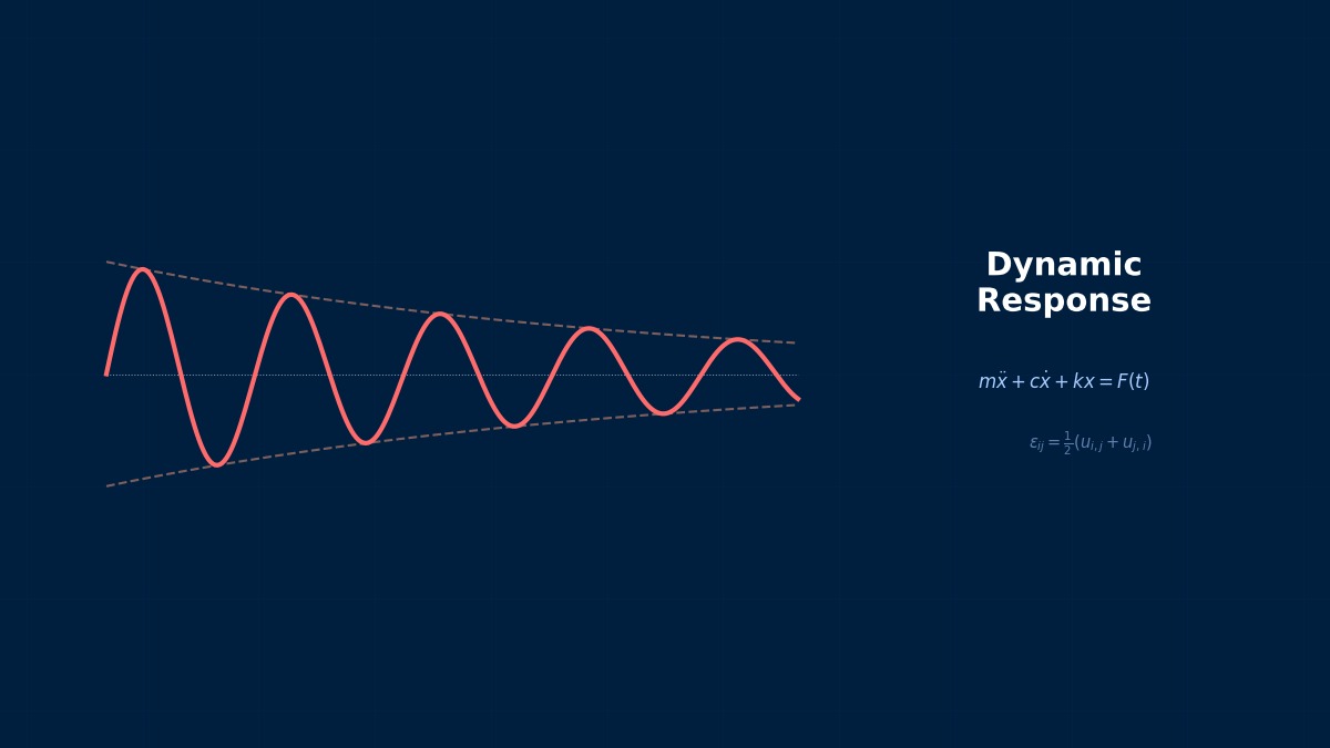
It is a simplified formula for random vibration of a single-degree-of-freedom system derived by John Miles (1954). When the input PSD is constant (white noise approximation), the RMS value of the response can be obtained with a single-line equation.
Or acceleration RMS:
Here $Q = 1/(2\zeta)$ is the quality factor of resonance, and $S_{\ddot{u}}(f_n)$ is the input acceleration PSD at the natural frequency.
It can be calculated in one line without FEM!
The Miles equation is ideal for screening evaluation. It provides a rough estimate before performing FEM PSD analysis to grasp the order of magnitude.
Assumptions and Limitations
Assumptions of the Miles equation:
1. Single-degree-of-freedom system — Cannot be directly applied to multi-degree-of-freedom systems
2. Input PSD is constant near the natural frequency — White noise approximation
3. Small damping — Approximately $\zeta < 0.1$
What happens if the input PSD is not constant?
Using the input PSD value at the natural frequency $f_n$ yields accuracy within 10-20% in many cases. It becomes inaccurate when the input PSD changes rapidly near $f_n$.
Practical Usage
Practical steps for using the Miles equation:
1. Estimate the equipment's first natural frequency $f_n$
2. Read the PSD value $S(f_n)$ from the vibration environment specification
3. Assume a damping ratio $\zeta$ (typically $\zeta = 0.02 \sim 0.05$)
4. Calculate the RMS response
5. Estimate the maximum response using 3σ (3×RMS)
6. Compare with allowable values
So there are situations where it can be used instead of FEM.
It is sufficient for screening during the conceptual design phase. For detailed design, proceed to FEM PSD analysis.
Summary
Key points:
- $a_{rms} = \sqrt{\pi f_n Q S(f_n) / 2}$ — A single-line formula
- Ideal for screening evaluation — Rough estimate before FEM
- White noise approximation — Input PSD is constant near $f_n$
- Use 3σ for maximum response — Can be used as a design value
- Not directly applicable to multi-degree-of-freedom systems — Can be applied individually to each mode
The Secret Story of the Miles Equation's Birth
The origin is the paper "On Structural Fatigue Under Random Loading" published by John W. Miles in 1954 in the Journal of the Aeronautical Sciences. Against the backdrop of the era when the U.S. Air Force struggled to predict aircraft fatigue failure, this groundbreaking formula was born under the bold assumptions of white noise approximation and a single-degree-of-freedom system, enabling the calculation of response RMS with just three parameters.
Computational Methods for Simple Evaluation Using Miles' Equation
Miles Equation Calculation Example
Please show me a specific calculation example.
Vibration evaluation of an electronic device's printed circuit board (PCB):
- $f_n = 200$ Hz (PCB's first natural frequency)
- $S_{\ddot{u}} = 0.04$ g²/Hz (Input PSD from MIL-STD-810)
- $Q = 20$ ($\zeta = 2.5\%$)
67 G acceleration! I'm worried if the BGA solder on the PCB can withstand that.
Typical shock resistance acceleration for BGA is 50-100 G. If the Miles equation gives 67 G, detailed evaluation with FEM is necessary. Consider PCB reinforcement or mounting changes.
Extension to Multi-Mode Systems
For multi-degree-of-freedom systems, apply Miles to each mode and combine using SRSS (Square Root of Sum of Squares):
Combine contributions from each mode using the square root of the sum of squares. Same as SRSS in response spectrum method, right?
SRSS combination is accurate if modes are sufficiently separated (approximately $f_{i+1}/f_i > 1.2$). For closely spaced modes, CQC (Complete Quadratic Combination) is required.
Summary
3-Step Calculation Method for Miles Equation
The application procedure for the Miles equation is 3 steps: ① Confirm natural frequency fn (Hz), ② Read the input PSD value G²/Hz (W(fn)) at fn, ③ Calculate response RMS = √(π/2 × fn × Q × W(fn)). The Q value (≈1/(2ζ)) is determined from the structural damping ratio ζ, typically assumed as Q=10 (ζ=5%) for aerospace structures. The calculation can be completed in 10 seconds even in Excel.
Simple Evaluation Using Miles' Equation in Practice
Miles Equation in Practice
Widely used for screening in random vibration evaluation of electronic equipment, space equipment, and military equipment.
Sensitivity Parameters
Parameters that most affect response in the Miles equation:
| Parameter | Effect on Response | Notes |
|---|---|---|
| $Q$ (Quality Factor) | $a_{rms} \propto \sqrt{Q}$ | If $Q$ doubles → RMS increases by $\sqrt{2}$ times |
| $f_n$ (Natural Frequency) | $a_{rms} \propto \sqrt{f_n}$ | Higher $f_n$ → Larger RMS |
| $S(f_n)$ (Input PSD) | $a_{rms} \propto \sqrt{S}$ | If input doubles → RMS increases by $\sqrt{2}$ times |
$Q$ (inverse of damping) is the most uncertain parameter, right?
Response changes by $\sqrt{5} \approx 2.2$ times between $Q = 10$ and $Q = 50$. The accuracy of damping estimation governs the accuracy of the Miles equation.
Practical Checklist
Related Topics
Experience the theory firsthand with the interactive simulator for this field
All Simulators