Random Vibration Fatigue

Category: 構造解析 | Integrated 2026-04-06
CAE visualization for random fatigue theory - technical simulation diagram
ランダム振動疲労

Theory and Physics

What is Random Vibration Fatigue?

🧑‍🎓

Professor, does fatigue occur under random vibration?


🎓

Random vibration is the repetition of irregular stress. The stress range fluctuates probabilistically, but damage accumulates cumulatively, leading to fatigue failure.


Fatigue Evaluation in the Frequency Domain

🎓

Instead of time-domain fatigue (Rainflow method + Miner's Rule), a method to directly estimate fatigue life from PSD:


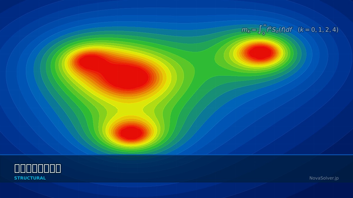
Dirlik Method (1985)

🎓

Estimates the probability density function (PDF) of stress ranges from the spectral moments of the stress PSD $S_{\sigma}(f)$, and calculates fatigue life using Miner's Rule.


$$ m_k = \int_0^\infty f^k S_{\sigma}(f) df \quad (k = 0, 1, 2, 4) $$

Constructs Dirlik's PDF from spectral moments $m_0, m_1, m_2, m_4$ and calculates the expected fatigue damage rate.


🧑‍🎓

So you can know the fatigue life without converting the PSD back to a time history!


🎓

The Dirlik method is reported to have good agreement with the time-domain Rainflow method. It handles broadband random stress and is a standard method for vibration fatigue evaluation.


Narrowband and Broadband Methods

🎓
MethodAssumptionAccuracy
NarrowbandStress is narrowband (dominated by a single resonance)Conservative (overestimates for broadband)
DirlikBroadband compatibleHigh (practical standard)
Benasciutti-TovoBroadband compatibleComparable to Dirlik
Zhao-BakerBroadband compatibleComparable to Dirlik

Summary

🎓

Key Points:


  • Directly estimate fatigue life from PSD — No need to convert back to time domain
  • Dirlik method is the practical standard — Handles broadband random stress
  • Spectral moments $m_0, m_1, m_2, m_4$ — Calculated from PSD integration
  • Vibration fatigue is an interdisciplinary field of NVH and fatigue — PSD analysis + fatigue evaluation

Coffee Break Yomoyama Talk

Palmgren-Miner Rule and Random Fatigue

The foundation of random fatigue life prediction is the linear cumulative damage rule proposed by Palmgren (1924) and Miner (1945). Failure is judged when the ratio Σ(ni/Ni) of the number of cycles ni at each stress amplitude Si to the fatigue life Ni at that Si (read from the S-N curve) reaches 1.0. However, the critical cumulative damage value for Miner's rule has a large experimental scatter of 0.3 to 3.0, and a 2009 survey by Cten reported an average of 0.7 (standard deviation 0.4) for carbon steel welded joints.

Physical Meaning of Each Term
  • Inertia Term (Mass Term): $\rho \ddot{u}$, i.e., "mass × acceleration". Have you ever experienced being thrown forward when slamming on the brakes? That "feeling of being pulled" is precisely the inertial force. Heavier objects are harder to set in motion and harder to stop once moving. Buildings shake during earthquakes because the ground moves suddenly while the building's mass "gets left behind". In static analysis, this term is set to zero, which assumes "forces are applied slowly enough that acceleration can be ignored". It absolutely cannot be omitted for impact loads or vibration problems.
  • Stiffness Term (Elastic Restoring Force): $Ku$ or $\nabla \cdot \sigma$. When you stretch a spring, you feel a "force trying to return it", right? That's Hooke's law $F=kx$, the essence of the stiffness term. So, a question—if you pull an iron rod and a rubber band with the same force, which stretches more? Obviously the rubber band. This "resistance to stretching" is the Young's modulus $E$, which determines stiffness. A common misconception: "high stiffness = strong" is incorrect. Stiffness is "resistance to deformation", strength is "resistance to failure"—they are different concepts.
  • External Force Term (Load Term): Body force $f_b$ (gravity, etc.) and surface force $f_s$ (pressure, contact force, etc.). Think of it this way—the weight of a truck on a bridge is a "force acting on the entire interior" (body force), while the force of the tires pushing on the road surface is a "force acting only on the surface" (surface force). Wind pressure, water pressure, bolt tightening force... all are external forces. A typical pitfall here: getting the load direction wrong. Intending "tension" but ending up with "compression"—it sounds like a joke, but it actually happens when coordinate systems are rotated in 3D space.
  • Damping Term: Rayleigh damping $C\dot{u} = (\alpha M + \beta K)\dot{u}$. Try plucking a guitar string. Does the sound continue forever? No, it gradually fades away. That's because vibration energy is converted to heat by air resistance and internal friction in the string. Car shock absorbers work on the same principle—they intentionally absorb vibration energy to improve ride comfort. What if damping were zero? Buildings would keep shaking forever after an earthquake. Since that doesn't happen in reality, setting appropriate damping is crucial.
Assumptions and Applicability Limits
  • Continuum assumption: Treats material as a continuous medium, ignoring microscopic heterogeneity.
  • Small deformation assumption (for linear analysis): Deformation is sufficiently small compared to initial dimensions, and the stress-strain relationship is linear.
  • Isotropic material (unless otherwise specified): Material properties are independent of direction (anisotropic materials require separate tensor definitions).
  • Quasi-static assumption (for static analysis): Ignores inertial and damping forces, considering only the balance between external and internal forces.
  • Non-applicable cases: For large deformation/large rotation problems, geometric nonlinearity is required. For nonlinear material behavior like plasticity or creep, constitutive law extensions are needed.
Dimensional Analysis and Unit Systems
VariableSI UnitNotes / Conversion Memo
Displacement $u$m (meter)When inputting in mm, unify loads and elastic modulus to MPa/N system
Stress $\sigma$Pa (Pascal) = N/m²MPa = 10⁶ Pa. Be careful of unit inconsistency when comparing with yield stress
Strain $\varepsilon$Dimensionless (m/m)Note the distinction between engineering strain and logarithmic strain (for large deformation)
Elastic Modulus $E$PaSteel: ~210 GPa, Aluminum: ~70 GPa. Note temperature dependence
Density $\rho$kg/m³In mm system: tonne/mm³ (= 10⁻⁹ tonne/mm³ for steel)
Force $F$N (Newton)Unify as N in mm system, N in m system

Numerical Methods and Implementation

Random Fatigue Calculation Procedure

🎓

1. FEM PSD Analysis — Calculate stress PSD $S_{\sigma}(f)$ at all nodes

2. Calculate Spectral Moments — $m_0, m_1, m_2, m_4$

3. Estimate PDF using Dirlik Method — Probability density function of stress ranges

4. Fatigue Damage using Miner's Rule — $D = \sum n_i / N_i$

5. Fatigue Life — $T = T_{test} / D$


Solver/Tools

🎓
ToolRandom Fatigue
nCode DesignLifeSupports Dirlik method. Directly inputs FEM results (PSD stress)
fe-safeDirlik method. Reads results from Abaqus/Nastran
FEMFATDirlik method. Automotive vibration fatigue standard
Nastran + PARAM,FATIGUELimited random fatigue capability
🧑‍🎓

So dedicated fatigue software is necessary.


🎓

FEM solvers themselves have limited random fatigue functionality. The standard workflow is to calculate PSD stress with FEM and evaluate life with dedicated fatigue software (nCode, fe-safe, FEMFAT).


Summary

🎓
  • FEM PSD analysis → Dirlik method in fatigue software — Standard workflow
  • nCode DesignLife / fe-safe / FEMFAT — Dedicated fatigue software
  • Estimate PDF from spectral moments — Damage using Miner's rule

  • Coffee Break Yomoyama Talk

    Rainflow Counting Method Implementation and Standards

    The Rainflow counting method is a stress amplitude counting algorithm jointly published in 1968 by Matsumoto Hiroshi (Kyoto University) and Yamada Michio, with the name inspired by the image of rain flowing down a roof. It is now standardized as ASTM E1049-85 (revised 1997). In Python, it can be implemented with the rainflow package (pip install rainflow), and counting for 10,000 points of time-history stress data completes in under 0.1 seconds. The counting result matrix display (From-To Matrix) is also a standard output in the MATLAB Fatigue Toolbox.

    Linear Elements (1st-order elements)

    Linear interpolation between nodes. Low computational cost but low stress accuracy. Beware of shear locking (mitigated with reduced integration or B-bar method).

    Quadratic Elements (with mid-side nodes)

    Can represent curved deformation. Stress accuracy improves significantly, but degrees of freedom increase by about 2-3 times. Recommended: when stress evaluation is critical.

    Full Integration vs Reduced Integration

    Full Integration: Risk of over-constraint (locking). Reduced Integration: Risk of hourglass modes (zero-energy modes). Choose appropriately for the situation.

    Adaptive Mesh

    Automatic refinement based on error indicators (e.g., ZZ estimator). Efficiently improves accuracy in stress concentration areas. Includes h-method (element subdivision) and p-method (order increase).

    Newton-Raphson Method

    Standard method for nonlinear analysis. Updates tangent stiffness matrix every iteration. Achieves quadratic convergence within convergence radius, but computational cost is high.

    Modified Newton-Raphson Method

    Updates tangent stiffness matrix at initial value or every few iterations. Cost per iteration is low, but convergence speed is linear.

    Convergence Criteria

    Force residual norm: $||R|| / ||F_{ext}|| < \epsilon$ (typically $\epsilon = 10^{-3}$ to $10^{-6}$). Displacement increment norm: $||\Delta u|| / ||u|| < \epsilon$. Energy norm: $\Delta u \cdot R < \epsilon$

    Load Increment Method

    Applies total load in small increments rather than all at once. The arc-length method (Riks method) can trace beyond extremum points on the load-displacement relationship.

    Analogy: Direct Method vs Iterative Method

    The direct method is like "solving simultaneous equations accurately with pen and paper"—reliable but takes too long for large-scale problems. The iterative method is like "repeatedly guessing to approach the correct answer"—starts with a rough answer but improves accuracy with each iteration. It's the same principle as looking up a word in a dictionary: it's more efficient to open it at an estimated location and adjust forward/backward (iterative method) than to search sequentially from the first page (direct method).

    Relationship Between Mesh Order and Accuracy

    1st-order elements are like "approximating a curve with a ruler"—represented by straight line segments, so accuracy is limited. 2nd-order elements are like a "flexible curve"—can represent curved changes, dramatically improving accuracy even at the same mesh density. However, computational cost per element increases, so judgment should be based on total cost-effectiveness.

    Practical Guide

    Random Fatigue in Practice

    🎓

    Random vibration fatigue is a problem in automotive exhaust systems (mufflers, catalytic converters), aircraft structures, and electronic device PCBs.


    Practical Checklist

    🎓
    • [ ] Is the stress PSD calculated correctly? (FEM PSD analysis results)
    • [ ] Is the S-N curve based on material test data?
    • [ ] Is the Dirlik method (or an appropriate broadband method) used?
    • [ ] Is the fatigue damage degree $D < 1$?
    • [ ] Is the stress concentration factor $K_t$ considered?
    • [ ] Is the effect of mean stress (Goodman, etc.) considered?

    • 🧑‍🎓
      関連シミュレーター

      この分野のインタラクティブシミュレーターで理論を体感しよう

      シミュレーター一覧

      関連する分野

      この記事の評価
      ご回答ありがとうございます!
      参考に
      なった
      もっと
      詳しく
      誤りを
      報告
      参考になった
      0
      もっと詳しく
      0
      誤りを報告
      0
      Written by NovaSolver Contributors
      Anonymous Engineers & AI — サイトマップ