Rainflow method (cycle counting)
Theory and Physics
What is the Rainflow Method?
Professor, what is the Rainflow Method?
Rainflow Counting is a technique to extract closed hysteresis loops (cycles) from a fluctuating load time history. It was named by Endo and Matsuishi (1968, Japan) by analogy to the flow of rainwater.
Why is Cycle Counting Necessary?
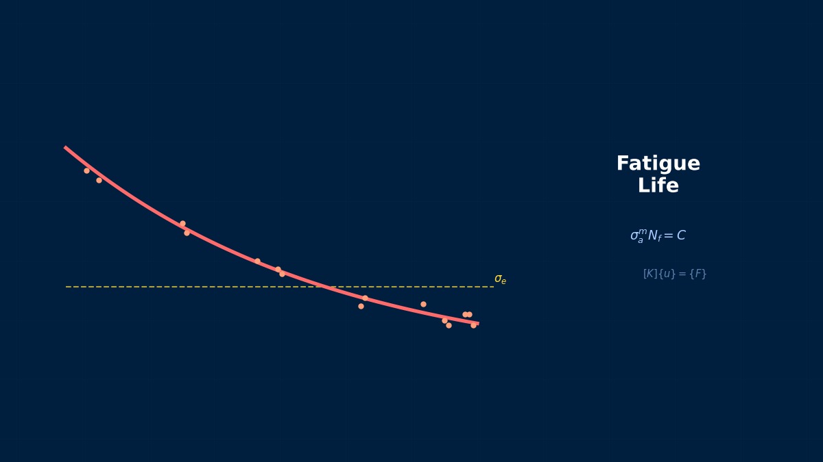
S-N curves and the Coffin-Manson equation give fatigue life for constant amplitude loading. Real loads are variable amplitude. The Rainflow Method decomposes variable loads into "a collection of many constant amplitude cycles," and cumulative damage is calculated using Miner's rule.
Algorithm
1. Extract peaks and valleys from the stress time history
2. Identify closed cycles as if "rainwater flows down a pagoda roof"
3. Record the stress range $\Delta\sigma$ and mean stress $\sigma_m$ for each cycle
4. Construct a histogram (Rainflow Matrix)
Summary
The "Rain Flowing Down a Roof" Algorithm
The name "Rainflow Method" comes from the fact that when the stress time history graph is rotated 90°, it resembles rainwater flowing down a roof. Proposed by Noboru Endo and Koji Matsuishi in 1968, it became a world standard as a method for accurately extracting fatigue cycles from irregular variable loads. It was standardized as ASTM E1049 in 1985.
Physical Meaning of Each Term
- Inertia Term (Mass Term): $\rho \ddot{u}$, meaning "mass × acceleration". Have you ever experienced being thrown forward during sudden braking? That "feeling of being carried away" is precisely the inertial force. Heavier objects are harder to set in motion and harder to stop once moving. Buildings shake during earthquakes because the ground moves suddenly while the building's mass "gets left behind". In static analysis, this term is set to zero, assuming "the force is applied slowly enough to ignore acceleration". It absolutely cannot be omitted in impact load or vibration problems.
- Stiffness Term (Elastic Restoring Force): $Ku$ or $\nabla \cdot \sigma$. When you pull a spring, you feel a "force trying to return it", right? That's Hooke's law $F=kx$, the essence of the stiffness term. Now a question—if you pull an iron rod and a rubber band with the same force, which stretches more? Obviously the rubber band. This "resistance to stretching" is the Young's modulus $E$, which determines stiffness. A common misconception: "High stiffness ≠ strong". Stiffness is "resistance to deformation", strength is "resistance to failure"—they are different concepts.
- External Force Term (Load Term): Body forces $f_b$ (gravity, etc.) and surface forces $f_s$ (pressure, contact force, etc.). Think of it this way—the weight of a truck on a bridge is a "force acting on the entire volume" (body force), while the force of the tires pushing on the road surface is a "force acting only on the surface" (surface force). Wind pressure, water pressure, bolt tightening force... all are external forces. A typical mistake here: getting the load direction wrong. Intending "tension" but ending up with "compression"—it sounds like a joke, but it actually happens when coordinate systems are rotated in 3D space.
- Damping Term: Rayleigh damping $C\dot{u} = (\alpha M + \beta K)\dot{u}$. Try plucking a guitar string. Does the sound continue forever? No, it gradually fades. That's because vibration energy is converted to heat by air resistance and internal friction in the string. Car shock absorbers work on the same principle—they intentionally absorb vibration energy to improve ride comfort. What if damping were zero? Buildings would keep shaking forever after an earthquake. Since that doesn't happen in reality, setting appropriate damping is crucial.
Assumptions and Applicability Limits
- Continuum assumption: Treats material as a continuous medium, ignoring microscopic heterogeneity
- Small deformation assumption (for linear analysis): Deformation is sufficiently small compared to initial dimensions, and the stress-strain relationship is linear
- Isotropic material (unless specified otherwise): Material properties are independent of direction (anisotropic materials require separate tensor definitions)
- Quasi-static assumption (for static analysis): Ignores inertial and damping forces, considering only the balance between external and internal forces
- Non-applicable cases: Large deformation/large rotation problems require geometric nonlinearity. Nonlinear material behavior like plasticity or creep requires constitutive law extensions
Dimensional Analysis and Unit Systems
| Variable | SI Unit | Notes / Conversion Memo |
|---|---|---|
| Displacement $u$ | m (meter) | When inputting in mm, unify load and elastic modulus to MPa/N system |
| Stress $\sigma$ | Pa (Pascal) = N/m² | MPa = 10⁶ Pa. Be careful of unit system inconsistency when comparing with yield stress |
| Strain $\varepsilon$ | Dimensionless (m/m) | Note the distinction between engineering strain and logarithmic strain (for large deformation) |
| Elastic modulus $E$ | Pa | Steel: ~210 GPa, Aluminum: ~70 GPa. Note temperature dependence |
| Density $\rho$ | kg/m³ | In mm system: tonne/mm³ (= 10⁻⁹ tonne/mm³ for steel) |
| Force $F$ | N (Newton) | Unify as N in mm system, N in m system |
Numerical Methods and Implementation
Rainflow Method Calculation
The Rainflow Method is built into all fatigue software. Input FEM stress time history → Rainflow → S-N/ε-N → Miner's rule automatic flow.
Also easily calculable in MATLAB/Python using the rainflow library.
Summary
How to Read a Rainflow Matrix
The result of the Rainflow Method is expressed as a Rainflow Matrix (RFC matrix), showing a frequency distribution with minimum stress on the vertical axis and maximum stress on the horizontal axis. Diagonal elements represent smaller amplitude, low cycle counts, while edge elements represent large amplitude, high damage cycles. Fatigue damage is dominated by elements far from the diagonal, and in actual evaluation, the accuracy of this edge data determines the accuracy of Miner's rule calculations.
Linear Elements (1st Order Elements)
Linear interpolation between nodes. Low computational cost but low stress accuracy. Beware of shear locking (mitigated by reduced integration or B-bar method).
Quadratic Elements (with Mid-side Nodes)
Can represent curved deformation. Stress accuracy improves significantly, but degrees of freedom increase by about 2-3 times. Recommended when stress evaluation is critical.
Full Integration vs Reduced Integration
Full Integration: Risk of over-constraint (locking). Reduced Integration: Risk of hourglass modes (zero-energy modes). Choose appropriately for the situation.
Adaptive Mesh
Automatic refinement based on error indicators (e.g., ZZ estimator). Efficiently improves accuracy in stress concentration areas. Includes h-method (element subdivision) and p-method (order increase).
Newton-Raphson Method
Standard method for nonlinear analysis. Updates tangent stiffness matrix every iteration. Shows quadratic convergence within convergence radius but has high computational cost.
Modified Newton-Raphson Method
Updates tangent stiffness matrix using initial value or every few iterations. Lower cost per iteration but linear convergence speed.
Convergence Criteria
Force residual norm: $||R|| / ||F_{ext}|| < \epsilon$ (typically $\epsilon = 10^{-3}$ to $10^{-6}$). Displacement increment norm: $||\Delta u|| / ||u|| < \epsilon$. Energy norm: $\Delta u \cdot R < \epsilon$
Load Increment Method
Applies the full load in small increments rather than all at once. The arc-length method (Riks method) can trace beyond extremum points on the load-displacement curve.
Analogy: Direct Method vs Iterative Method
The direct method is like "solving simultaneous equations accurately with pen and paper"—reliable but takes too long for large-scale problems. The iterative method is like "repeatedly guessing to approach the correct answer"—starts with a rough answer but improves accuracy with each iteration. It's the same principle as looking up a word in a dictionary: it's more efficient to estimate where to open it and adjust forward/backward (iterative method) than to search sequentially from the first page (direct method).
Relationship Between Mesh Order and Accuracy
1st order elements are like "approximating a curve with a ruler"—represented by straight line segments, so accuracy is limited. 2nd order elements are like a "flexible curve"—can represent curved changes, dramatically improving accuracy even at the same mesh density. However, computational cost per element increases, so judge based on total cost-effectiveness.
Practical Guide
Rainflow Method in Practice
Evaluating fatigue life from automotive road data (real driving stress time history). Aircraft flight spectra. Pressure cycles in piping.
Practical Checklist
Fatigue Evaluation from Real Road Data
In automotive durability testing, real road driving data is measured with strain gauges and analyzed using the Rainflow Method to evaluate fatigue damage. Ford standardized this approach with EDAP (Engineering Durability Analysis Package) in the 1980s, optimizing an algorithm that could process data from 10km of Belgian road driving in just seconds on 1990s PCs.
Analogy for the Analysis Flow
The analysis flow is actually very similar to cooking. First, buy ingredients (prepare CAD model), do the prep work (mesh generation), apply heat (solver execution), and finally plate it (visualization in post-processing). Here's an important question—in cooking, which step is most prone to failure? Actually, it's the "prep work". If mesh quality is poor, the results will be a mess no matter how excellent the solver is.
Pitfalls Beginners Often Fall Into
Are you checking mesh convergence? Do you think "the calculation ran = the result is correct"? This is actually the most common trap for CAE beginners. The solver will always return "some answer" for the given mesh. But if the mesh is too coarse, that answer will be far from reality. Confirm that results stabilize across at least three levels of mesh density—neglecting this leads to the dangerous assumption that "the computer gave the answer, so it must be correct."
Thinking About Boundary Conditions
Setting boundary conditions is like "writing the problem statement" for an exam. If the problem statement is wrong? No matter how accurately you calculate, the answer will be wrong. "Is this surface really fully fixed?" "Is this load really uniformly distributed?"—Correctly modeling real constraint conditions is actually the most critical step in the entire analysis.
Software Comparison
Tools
Built into all fatigue software. Also possible in MATLAB/Python.
Standard Differences and Implementation of Rainflow Counting
Cycle counting results for the same load history can differ by up to 15% between ASTM E1049-85 and DIN 45667. MSC Fatigue defaults to the 4-point method (ASTM compliant), nCode defaults to the HCM method (DIN compliant), and the automotive industry standard at ZF is the HCM method. Standard selection directly impacts fatigue life prediction accuracy.
The Three Most Important Questions for Selection
- "What are you solving?": Does the required physical model/element type for the Rainflow Method (cycle counting) have support? For example, presence of LES support for fluids, contact/large deformation capability for structures makes a difference.
- "Who will use it?": For beginner teams, tools with rich GUI are suitable; for experienced users, flexible script-driven tools are better. Similar to the difference between automatic (GUI) and manual (script) transmission cars.
- "How far will it be extended?": Selection considering future analysis scale expansion (HPC support), deployment to other departments, and integration with other tools leads to long-term cost reduction.
Advanced Technology
Advanced Rainflow Method
Extension to Gaussian Processes and Non-stationary Loads
Traditional Rainflow Method assumes stationary random loads, but actual loads are often non-stationary processes where statistical properties change over time. The "windowed Rainflow Method" established in the 2010s performs cycle extraction within time windows, enabling handling of non-stationary loads. Applied to fatigue evaluation of wind turbines due to changing operating conditions.
Troubleshooting
Rainflow Method Troubles
Residual Cycle Problem with Truncated Data
When the beginning and end of measured data are incomplete, "residual" cycles occur in the Rainflow Method. Ignoring these leads to 10-20% underestimation of damage. ASTM E1049 recommends complementing residual cycles using the range-pair method, but in practice, designing the measurement protocol so the entire measurement interval is complete is the fundamental solution.
When You Think "The Analysis Doesn't Match"
- First, take a deep breath—Panicking and randomly changing settings makes the problem more complex.
- Create a minimal reproducible case—Reproduce the Rainflow Method (cycle counting) problem in its simplest form. "Subtractive debugging" is most efficient.
- Change one thing and re-run—Making multiple changes simultaneously makes it unclear what worked. The principle of "controlled experiment" same as in science.
- Return to physics—If the calculation result is non-physical, like "objects floating against gravity", suspect fundamental mistakes in input data.
Related Topics
なった
詳しく
報告