Vibration Test Simulation

Category: 構造解析 | Integrated 2026-04-06
CAE visualization for vibration testing theory - technical simulation diagram
振動試験シミュレーション

Theory and Physics

What is Vibration Test Simulation?

🧑‍🎓

Professor, what is the purpose of conducting FEM simulation for vibration tests?


🎓

Two purposes:


1. Pre-test Risk Assessment — Identify the risk of failure due to resonance beforehand

2. Optimization of Test Conditions — Review excessive test conditions (prevention of over-testing)


Types of Vibration Tests

🎓
Test TypeInputPurposeStandards
Sinusoidal SweepSine wave (frequency sweep)Understanding resonance characteristicsMIL-STD-810
Random VibrationPSD InputReplication of actual usage environmentMIL-STD-810, IEC 60068
Shock TestSRS or Half-sine waveVerification of shock resistanceMIL-STD-810
Sine BurstBurst of sine wavesVerification of response at resonanceInternal company standards

Replication in FEM

🎓

Replicate the state mounted on a vibration test shaker in FEM:

1. Modeling of the Fixture — Fixture connecting the test specimen and the shaker

2. Base Excitation Input — Acceleration input from the shaker

3. Frequency Response or Time History Analysis — Depending on test conditions

4. Response Evaluation — Maximum values of acceleration, stress, displacement


🧑‍🎓

Do we also model the fixture?


🎓

If the natural frequency of the fixture falls within the test frequency band, the fixture's resonance affects the test results. Model the fixture to check for fixture resonance beforehand.


Summary

🎓

Key Points:


  • Pre-test risk assessment and condition optimization — The two purposes of FEM
  • Sinusoidal sweep / Random / Shock — The three main test types
  • Fixture modeling is important — Be cautious of fixture resonance
  • MIL-STD-810, IEC 60068 — Major vibration test standards

Coffee Break Yomoyama Talk

Theoretical Background of Vibration Test Standards

Many vibration test standards are established by statistically processing measured PSD data from actual usage environments. MIL-STD-810G (2008) is a US Department of Defense environmental test standard for military equipment, categorizing transport/usage environments into 10 PSD profile categories. The "Taylor Category C (Ground Vehicles)" shown in Annex C specifies a test level of 0.04 G²/Hz from 20 to 500Hz. However, the concept of safety factors differs between IEC 60068 and MIL-STD, and some harmonization is progressing through international harmonization (2016 revision of IEC 60721-3).

Physical Meaning of Each Term
  • Inertia Term (Mass Term): $\rho \ddot{u}$, meaning "mass × acceleration". Haven't you experienced your body being thrown forward during sudden braking? That "feeling of being pulled" is precisely the inertial force. Heavier objects are harder to set in motion and harder to stop once moving. Buildings shake during earthquakes because the ground moves suddenly while the building's mass is "left behind". In static analysis, this term is set to zero, assuming "acceleration can be ignored because the force is applied slowly". It absolutely cannot be omitted in shock loads or vibration problems.
  • Stiffness Term (Elastic Restoring Force): $Ku$ or $\nabla \cdot \sigma$. When you pull a spring, you feel a "force trying to return it", right? That is Hooke's law $F=kx$, the essence of the stiffness term. Now a question — an iron rod and a rubber band, which stretches more when pulled with the same force? Obviously the rubber. This "resistance to stretching" is the Young's modulus $E$, which determines stiffness. A common misconception: "High stiffness ≠ strong". Stiffness is "resistance to deformation", strength is "resistance to failure" — different concepts.
  • External Force Term (Load Term): Body force $f_b$ (gravity, etc.) and surface force $f_s$ (pressure, contact force, etc.). Think of it this way — the weight of a truck on a bridge is a "force acting on the entire volume" (body force), the force of the tire pushing on the road is a "force acting only on the surface" (surface force). Wind pressure, water pressure, bolt tightening force... all are external forces. A typical mistake here: getting the load direction wrong. Intending "tension" but it becomes "compression" — sounds like a joke, but it actually happens when coordinate systems are rotated in 3D space.
  • Damping Term: Rayleigh damping $C\dot{u} = (\alpha M + \beta K)\dot{u}$. Try plucking a guitar string. Does the sound continue forever? No, it gradually fades. That's because vibration energy is converted to heat by air resistance and internal friction in the string. Car shock absorbers work on the same principle — intentionally absorbing vibration energy to improve ride comfort. What if damping were zero? Buildings would continue shaking forever after an earthquake. Since that doesn't happen in reality, setting appropriate damping is crucial.
Assumptions and Applicability Limits
  • Continuum assumption: Treats material as a continuous medium, ignoring microscopic heterogeneity
  • Small deformation assumption (for linear analysis): Deformation is sufficiently small compared to initial dimensions, stress-strain relationship is linear
  • Isotropic material (unless otherwise specified): Material properties are independent of direction (anisotropic materials require separate tensor definition)
  • Quasi-static assumption (for static analysis): Ignores inertial/damping forces, considers only equilibrium between external and internal forces
  • Non-applicable cases: Large deformation/large rotation problems require geometric nonlinearity. Nonlinear material behavior like plasticity or creep requires constitutive law extension
Dimensional Analysis and Unit Systems
VariableSI UnitNotes / Conversion Memo
Displacement $u$m (meter)When inputting mm, unify loads/elastic modulus to MPa/N system
Stress $\sigma$Pa (Pascal) = N/m²MPa = 10⁶ Pa. Be careful of unit system inconsistency when comparing with yield stress
Strain $\varepsilon$Dimensionless (m/m)Note the distinction between engineering strain and logarithmic strain (for large deformation)
Elastic Modulus $E$PaSteel: ~210 GPa, Aluminum: ~70 GPa. Note temperature dependence
Density $\rho$kg/m³In mm system: tonne/mm³ (= 10⁻⁹ tonne/mm³ for steel)
Force $F$N (Newton)Unify as N in mm system, N in m system

Numerical Methods and Implementation

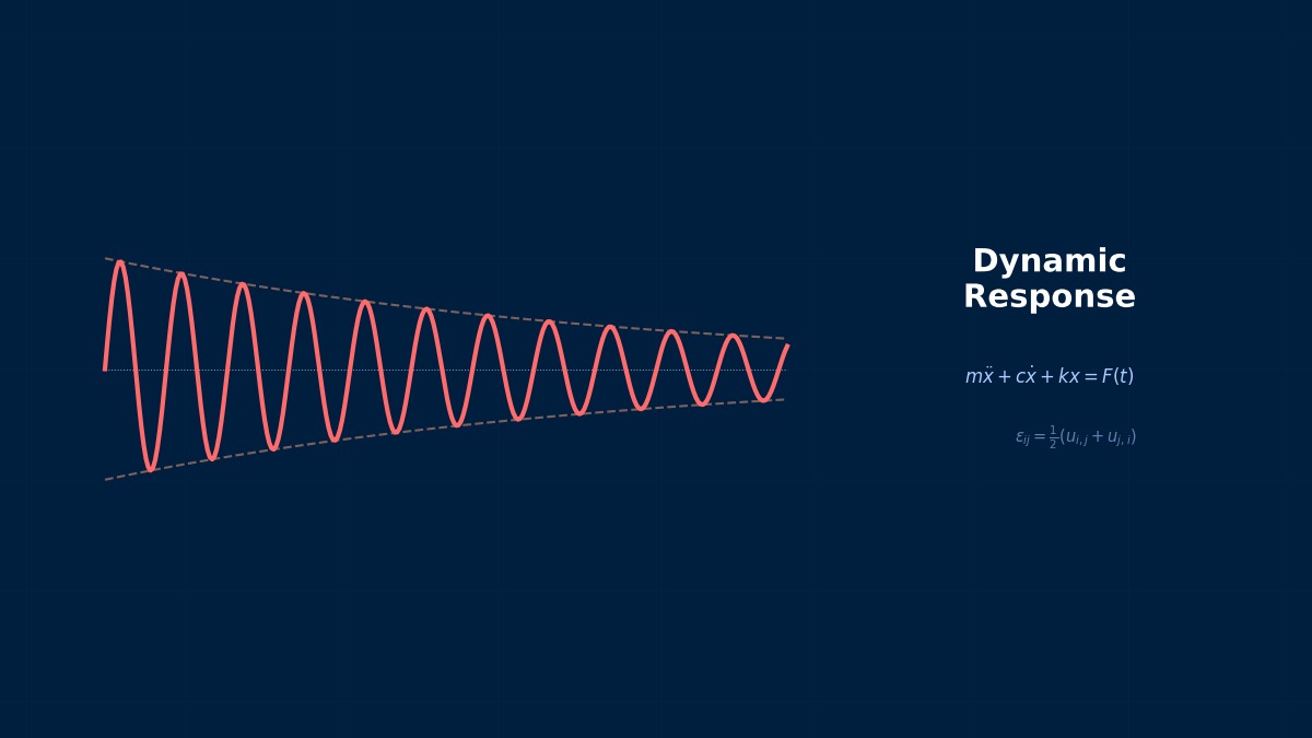
FEM for Sinusoidal Sweep

🎓

Sinusoidal Sweep = Frequency Response Analysis:


Nastran

```

SOL 111

CEND

METHOD = 10

FREQUENCY = 20

DLOAD = 100

```

Input acceleration as base excitation with frequency sweep.

FEM for Random Vibration

```

SOL 111

CEND

RANDOM = 20

```

Random response with PSD input.

Acceleration Response Evaluation

🎓

Main evaluation items for test results:


ItemSinusoidal SweepRandom
Peak AccelerationFRF peak value × input3σ (3×RMS)
Resonance FrequencyFRF peak location
StressStress conversion from FRF3σ stress

Summary

🎓
  • Sinusoidal Sweep = Frequency Response (SOL 111)
  • Random = PSD Response (SOL 111 + RANDOM)
  • Shock = Time History (SOL 112) → SRS
  • Analyze with full model including fixture

  • Coffee Break Yomoyama Talk

    Mechanism of Shaker Control Loop

    Control of random vibration tests using electrodynamic shakers is a closed-loop process: ① Set reference PSD (Target PSD), ② Controller corrects shaker dynamics via inverse system identification (FRF measurement), ③ Drive signal is iteratively updated so that the PSD at the control point (usually an accelerometer on the mounting table) converges to the target value. Convergence criteria are generally ±3dB RMS error, and the time to achieve 1Hz resolution control averages 20–60 seconds. The Vibration Research VR9500 controller's convergence algorithm is considered among the fastest in the industry.

    Linear Elements (1st-order elements)

    Linear interpolation between nodes. Low computational cost but low stress accuracy. Beware of shear locking (mitigated by reduced integration or B-bar method).

    Quadratic Elements (with mid-side nodes)

    Can represent curved deformation. Stress accuracy improves significantly, but degrees of freedom increase by about 2–3 times. Recommended: when stress evaluation is critical.

    Full Integration vs Reduced Integration

    Full Integration: Risk of over-constraint (locking). Reduced Integration: Risk of hourglass modes (zero-energy modes). Choose appropriately.

    Adaptive Mesh

    Automatic refinement based on error indicators (e.g., ZZ estimator). Efficiently improves accuracy in stress concentration areas. Includes h-method (element subdivision) and p-method (order increase).

    Newton-Raphson Method

    Standard method for nonlinear analysis. Updates tangent stiffness matrix each iteration. Quadratic convergence within convergence radius, but high computational cost.

    Modified Newton-Raphson Method

    Updates tangent stiffness matrix using initial value or every few iterations. Lower cost per iteration, but convergence is linear.

    Convergence Criteria

    Force residual norm: $||R|| / ||F_{ext}|| < \epsilon$ (typically $\epsilon = 10^{-3}$〜$10^{-6}$). Displacement increment norm: $||\Delta u|| / ||u|| < \epsilon$. Energy norm: $\Delta u \cdot R < \epsilon$

    Load Increment Method

    Applies total load incrementally in small steps rather than all at once. The arc-length method (Riks method) can trace beyond extremum points on the load-displacement curve.

    Analogy: Direct Method vs Iterative Method

    The direct method is like "solving simultaneous equations accurately with pen and paper" — reliable but takes too long for large-scale problems. The iterative method is like "repeatedly guessing to approach the correct answer" — starts with a rough answer but accuracy improves with each iteration. It's the same principle as looking up a word in a dictionary: it's more efficient to estimate and open near it, then adjust forward/backward (iterative method) than to search sequentially from the first page (direct method).

    Relationship Between Mesh Order and Accuracy

    1st-order elements are like "approximating a curve with a ruler" — represented by straight line segments, so accuracy is limited. 2nd-order elements are like "flexible curves" — can represent curved changes, dramatically improving accuracy even at the same mesh density. However, computational cost per element increases, so judge based on total cost-effectiveness.

    Practical Guide

    Prevention of Over-testing (Force Limiting)

    🎓

    In vibration tests, differences in impedance between the test article and the shaker can cause inputs greater than the actual environment (over-testing). Calculate the actual environmental input with FEM and optimize test conditions (Force Limiting). The method is specified in NASA-HDBK-7004.


    🧑‍🎓

    So test conditions can sometimes be more severe than the actual environment?


    🎓

    The test shaker is an "ideal rigid wall", but the actual mounting state (e.g., upper stage of a rocket) is a "flexible structure". Applying the rigid shaker's input to equipment mounted on a flexible structure can cause resonance response to be many times greater than in the actual environment. Calculate the mounted impedance with FEM and notch (cut out) the test conditions.


    Practical Checklist

    🎓
    • [ ] Are test conditions (PSD, sine wave, shock) compliant with standards?
    • [ ] Is the fixture model included?
    • [ ] Is the fixture's natural frequency outside the test band?
    • [ ] Has the risk of over-testing been assessed?
    • [ ] Has the need for Force Limiting been considered?
    • [ ] Is the 3σ response within the allowable limits of components?

    • 🧑‍🎓

      So "prevention of over-testing" is one of the important purposes of FEM simulation.


      🎓

      Failure of test articles is costly. Optimizing test conditions beforehand with FEM can prevent unnecessary failures due to over-testing.


      Coffee Break Yomoyama Talk

      Vibration Test Certification Process for Automotive ECUs

      Vibration test certification for automotive ECUs (Engine Control Units) is conducted in accordance with ISO 16750-3. Products mounted in the engine compartment require combined sine + random tests of Category M (10–2000Hz, including engine components), with a test duration of 96 hours per axis. Bosch's DE10-type ECU completed the Category M2 equivalent test (RMS 22G) at BMW's certification test facility in 2022 and was adopted for the BMW 5 Series (G60 model). Test costs typically range from 2 to 5 million yen per lot (3 samples).

      Analogy: Analysis Flow

      The analysis flow is actually very similar to cooking. First, buy ingredients (prepare CAD model), do the prep work (mesh generation), apply heat (solver execution), and finally plate it (visualization in post-processing). Here's an important question — which step in cooking is most prone to failure? Actually, it's the "prep work". If mesh quality is poor, the results will be a mess no matter how excellent the solver is.

      Common Pitfalls for Beginners

      Are you checking mesh convergence? Do you think "the calculation ran = the result is correct"? This is actually the most common trap for CAE beginners. The solver will always return "some answer" for the given mesh...

      関連シミュレーター

      この分野のインタラクティブシミュレーターで理論を体感しよう

      シミュレーター一覧

      関連する分野

      熱解析製造プロセス解析V&V・品質保証
      この記事の評価
      ご回答ありがとうございます!
      参考に
      なった
      もっと
      詳しく
      誤りを
      報告
      参考になった
      0
      もっと詳しく
      0
      誤りを報告
      0
      Written by NovaSolver Contributors
      Anonymous Engineers & AI — サイトマップ
      About the Authors