Crack Initiation Life Prediction
Theory and Physics
What is Crack Initiation Life?
Professor, is fatigue life divided into "crack initiation" and "crack propagation"?
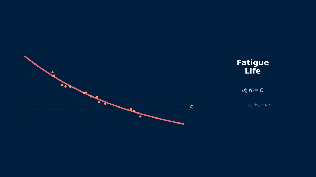
Total Life = Crack Initiation Life ($N_i$) + Crack Propagation Life ($N_p$). The S-N method and Coffin-Manson method mainly predict crack initiation life. Propagation after crack initiation is evaluated by Paris' law (fracture mechanics).
Crack Initiation Mechanism
1. Formation of Slip Bands — Persistent slip bands (PSB) form due to repeated plastic deformation.
2. Nucleation of Microcracks — Microcracks (several μm to tens of μm) from surface roughness in PSBs.
3. Growth of Short Cracks — Growth of short cracks at the grain level.
4. Transition to Long Cracks — Reaching a size where fracture mechanics becomes applicable ($\sim$ 1 mm).
Crack Initiation vs. Crack Propagation
| Characteristic | Crack Initiation | Crack Propagation |
|---|---|---|
| Size | < 1 mm | > 1 mm |
| Evaluation Method | S-N, ε-N, Multiaxial Fatigue | Paris' Law, $da/dN = C(\Delta K)^m$ |
| Proportion of Total Life | 80–90% in high-cycle fatigue | Important in low-cycle fatigue |
| Role of FEM | Stress/Strain Calculation | SIF ($\Delta K$) Calculation |
Summary
The Lesson of the de Havilland Comet
In 1954, the world's first jet airliner, the Comet, disintegrated in mid-air. The cause was crack initiation at stress concentrations in the corners of the windows. The stress at the corners reached three times the average under the same load, and fatal cracks formed in only about 3000 cycles. This accident made the world aware of the importance of crack initiation life analysis.
Physical Meaning of Each Term
- Inertia Term (Mass Term): $\rho \ddot{u}$, i.e., "mass × acceleration". Have you ever experienced being thrown forward when braking suddenly? That "feeling of being carried away" is precisely the inertial force. Heavier objects are harder to set in motion and harder to stop once moving. Buildings shake during earthquakes because the ground moves suddenly while the building's mass "gets left behind". In static analysis, this term is set to zero, assuming "forces are applied slowly so acceleration is negligible". It cannot be omitted in impact loads or vibration problems.
- Stiffness Term (Elastic Restoring Force): $Ku$ or $\nabla \cdot \sigma$. When you stretch a spring, you feel a "force trying to return it", right? That is Hooke's law $F=kx$, the essence of the stiffness term. Now a question—if you pull an iron rod and a rubber band with the same force, which stretches more? Obviously, the rubber band. This "resistance to stretching" is the Young's modulus $E$, which determines stiffness. A common misconception: "High stiffness ≠ strong". Stiffness is "resistance to deformation", strength is "resistance to failure"—different concepts.
- External Force Term (Load Term): Body forces $f_b$ (e.g., gravity) and surface forces $f_s$ (pressure, contact forces). Think of it this way—the weight of a truck on a bridge is a "force acting on the entire volume" (body force), while the force of the tires pushing on the road is a "force acting only on the surface" (surface force). Wind pressure, water pressure, bolt tightening force... all are external forces. A common mistake here: getting the load direction wrong. Intending "tension" but modeling "compression"—sounds like a joke, but it actually happens when coordinate systems rotate in 3D space.
- Damping Term: Rayleigh damping $C\dot{u} = (\alpha M + \beta K)\dot{u}$. Try plucking a guitar string. Does the sound continue forever? No, it gradually fades. That's because vibrational energy is converted to heat by air resistance and internal friction in the string. Car shock absorbers work on the same principle—they intentionally absorb vibrational energy for a smoother ride. What if damping were zero? Buildings would keep shaking forever after an earthquake. Since that doesn't happen in reality, setting appropriate damping is crucial.
Assumptions and Applicability Limits
- Continuum Assumption: Treats material as a continuous medium, ignoring microscopic inhomogeneities.
- Small Deformation Assumption (for linear analysis): Deformation is sufficiently small compared to initial dimensions, and the stress-strain relationship is linear.
- Isotropic Material (unless specified otherwise): Material properties are independent of direction (anisotropic materials require separate tensor definitions).
- Quasi-static Assumption (for static analysis): Ignores inertial and damping forces, considering only equilibrium between external and internal forces.
- Non-applicable Cases: Large deformation/large rotation problems require geometric nonlinearity. Nonlinear material behavior like plasticity or creep requires constitutive law extensions.
Dimensional Analysis and Unit Systems
| Variable | SI Unit | Notes / Conversion Memo |
|---|---|---|
| Displacement $u$ | m (meter) | When inputting in mm, unify load and elastic modulus to MPa/N system. |
| Stress $\sigma$ | Pa (Pascal) = N/m² | MPa = 10⁶ Pa. Be careful of unit inconsistency when comparing with yield stress. |
| Strain $\varepsilon$ | Dimensionless (m/m) | Note the distinction between engineering strain and logarithmic strain (for large deformations). |
| Elastic Modulus $E$ | Pa | Steel: ~210 GPa, Aluminum: ~70 GPa. Note temperature dependence. |
| Density $\rho$ | kg/m³ | In mm system: tonne/mm³ (= 10⁻⁹ tonne/mm³ for steel). |
| Force $F$ | N (Newton) | Unify as N in mm system, N in m system. |
Numerical Methods and Implementation
FEM for Crack Initiation
1. Calculate stress/strain with FEM — Elastic or elasto-plastic.
2. Evaluate crack initiation life with fatigue software — S-N method or ε-N method.
3. Perform crack propagation analysis if necessary — Crack growth with XFEM or CZM.
Summary
The Surprising Discoverer of the S-N Curve
The origin of fatigue life, the S-N curve, was established in the 1860s by the German railway engineer Wöhler. While investigating axle failures, he conducted repeated tests from 100,000 to 10 million cycles, quantitatively relating stress amplitude and cycles to failure for the first time. This painstaking data collection became the foundation of crack initiation life analysis.
Linear Elements (1st-order Elements)
Linear interpolation between nodes. Low computational cost but lower stress accuracy. Beware of shear locking (mitigated by reduced integration or B-bar method).
Quadratic Elements (with Mid-side Nodes)
Can represent curved deformation. Stress accuracy improves significantly, but degrees of freedom increase by about 2–3 times. Recommended when stress evaluation is critical.
Full Integration vs Reduced Integration
Full Integration: Risk of over-constraint (locking). Reduced Integration: Risk of hourglass modes (zero-energy modes). Choose appropriately.
Adaptive Mesh
Automatic refinement based on error indicators (e.g., ZZ estimator). Efficiently improves accuracy in stress concentration areas. Includes h-method (element subdivision) and p-method (order increase).
Newton-Raphson Method
Standard method for nonlinear analysis. Updates tangent stiffness matrix each iteration. Quadratic convergence within convergence radius, but high computational cost.
Modified Newton-Raphson Method
Updates tangent stiffness matrix using initial value or every few iterations. Lower cost per iteration, but convergence is linear.
Convergence Criteria
Force residual norm: $||R|| / ||F_{ext}|| < \epsilon$ (typically $\epsilon = 10^{-3}$ to $10^{-6}$). Displacement increment norm: $||\Delta u|| / ||u|| < \epsilon$. Energy norm: $\Delta u \cdot R < \epsilon$.
Load Increment Method
Applies total load in small increments rather than all at once. The arc-length method (Riks method) can track beyond limit points on the load-displacement curve.
Analogy: Direct Method vs. Iterative Method
The direct method is like "solving simultaneous equations accurately with pen and paper"—reliable but takes too long for large-scale problems. The iterative method is like "repeatedly guessing to approach the correct answer"—starts with a rough answer but improves accuracy with each iteration. It's the same principle as looking up a word in a dictionary: it's more efficient to estimate where to open it and adjust forward/backward (iterative) than to search sequentially from the first page (direct).
Relationship Between Mesh Order and Accuracy
1st-order elements are like "approximating a curve with a ruler"—represented by straight line segments, so accuracy is limited. 2nd-order elements are like "flexible curves"—can represent curved changes, dramatically improving accuracy even at the same mesh density. However, computational cost per element increases, so judge based on total cost-effectiveness.
Practical Guide
Crack Initiation in Practice
Evaluate using crack initiation life during the design stage. Use crack propagation life (determining inspection intervals) during inspection/maintenance.
Practical Checklist
Fatigue Design of Automotive Door Hinges
Automotive door hinges must withstand about 300,000 opening/closing cycles over their lifetime. In practice, crack initiation life analysis considering stress concentration factor Kt is used to evaluate areas around hinge holes. Since the 1990s, Toyota has established a method combining FEM and fatigue analysis to complete designs without prototyping.
Analogy of the Analysis Flow
The analysis flow is actually very similar to cooking. First, buy ingredients (prepare CAD model), do prep work (mesh generation), apply heat (solver execution), and finally plate it (visualization in post-processing). Here's an important question—which step in cooking is most prone to failure? Actually, it's the "prep work". If mesh quality is poor, results will be a mess no matter how good the solver is.
Pitfalls Beginners Often Fall Into
Are you checking mesh convergence? Do you think "the calculation ran = the result is correct"? This is actually the most common trap for CAE beginners. The solver will always return "some answer" for the given mesh. But if the mesh is too coarse, that answer can be far from reality. Confirm that results stabilize across at least three mesh density levels—neglecting this leads to the dangerous assumption that "the computer gave the answer, so it must be correct".
Thinking About Boundary Conditions
Setting boundary conditions is like "writing the problem statement" for an exam. If the problem statement is wrong? No matter how accurately you calculate, the answer will be wrong. "Is this surface really fully fixed?" "Is this load really uniformly distributed?"—Correctly modeling real-world constraints is often the most critical step in the entire analysis.
Software Comparison
Tools
fe-safe's Hot Spot Detection Feature
Dassault fe-safe automatically extracts the Hot Spots with the highest fatigue crack initiation risk from all FEM nodes and calculates crack initiation life in bulk by combining them with S-N curves. Since the late 2000s, it has been standardly adopted for ABS ship welding analysis, processing tens of thousands of nodes per model in minutes.
The Three Most Important Questions for Selection
- "What are you solving?": Does it support the physical models/element types needed for crack initiation life prediction? For example, presence of LES support for fluids, contact/large deformation capability for structures makes a difference.
- "Who will use it?": For beginner teams, tools with rich GUI are suitable; for experienced users, flexible script-driven tools are better. Similar to the difference between automatic (GUI) and manual (script) transmission cars.
- "How far will you expand?": Choosing with future expansion in mind—scaling up analysis (HPC support), deployment to other departments, integration with other tools—leads to long-term cost reduction.
Advanced Technologies
Advanced Topics in Crack Initiation
Related Topics
なった
詳しく
報告