確率論的破壊力学
Theory and Physics
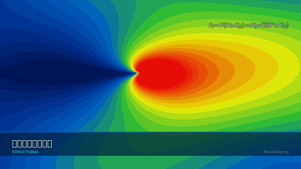
What is Probabilistic Fracture Mechanics?
Professor, what is probabilistic fracture mechanics?
Deterministic fracture mechanics uses a binary criterion: "fracture occurs if $K \geq K_{IC}$". Probabilistic fracture mechanics treats variations in crack size, material properties, and load as random variables to calculate the probability of fracture.
It evaluates "what is the probability of fracture in percent?" rather than "will it fracture or not?".
Used in nuclear power probabilistic risk assessment (PRA), aircraft damage tolerance, and pipeline reliability design.
Random Variables
| Parameter | Source of Variation |
|---|---|
| Crack Size $a$ | Inspection uncertainty, initial defect distribution |
| $K_{IC}$ | Variation between material lots |
| Load $\sigma$ | Variation in operating conditions |
| Paris Constants $C, m$ | Variation in material testing |
Calculation Methods
Summary
The Meaning of a 1/1000 Fracture Probability
In probabilistic fracture mechanics, an allowable fracture probability Pf=10⁻⁶ to 10⁻⁴ is set, and safety margins are evaluated considering variations in defect size and material toughness. The IAEA standard for nuclear pressure vessels requires Pf<10⁻⁶/year, which is a strict criterion meaning "no fracture occurs even with 1 million vessels operating for 1 year". The standard procedure is to evaluate using the Monte Carlo method with 10⁷ samples.
Physical Meaning of Each Term
- Inertia Term (Mass Term): $\rho \ddot{u}$, i.e., "mass × acceleration". Have you ever experienced being thrown forward when slamming on the brakes? That "feeling of being carried away" is precisely the inertial force. Heavier objects are harder to set in motion and harder to stop once moving. Buildings shake during earthquakes because the ground moves suddenly while the building's mass "gets left behind". In static analysis, this term is set to zero, assuming "forces are applied slowly enough that acceleration can be ignored". It absolutely cannot be omitted for impact loads or vibration problems.
- Stiffness Term (Elastic Restoring Force): $Ku$ or $\nabla \cdot \sigma$. When you stretch a spring, you feel a "force trying to return it", right? That's Hooke's law $F=kx$, the essence of the stiffness term. So here's a question—if you pull an iron rod and a rubber band with the same force, which stretches more? Obviously the rubber band. This "resistance to stretching" is the Young's modulus $E$, which determines stiffness. A common misconception: "high stiffness ≠ strong". Stiffness is "resistance to deformation", strength is "resistance to failure"—they are different concepts.
- External Force Term (Load Term): Body forces $f_b$ (e.g., gravity) and surface forces $f_s$ (pressure, contact forces). Think of it this way—the weight of a truck on a bridge is a "force acting on the entire volume" (body force), while the force of the tires pushing on the road surface is a "force acting only on the surface" (surface force). Wind pressure, water pressure, bolt tightening force... all are external forces. A common mistake here: getting the load direction wrong. Intending "tension" but modeling "compression"—sounds like a joke, but it actually happens when coordinate systems rotate in 3D space.
- Damping Term: Rayleigh damping $C\dot{u} = (\alpha M + \beta K)\dot{u}$. Try plucking a guitar string. Does the sound continue forever? No, it gradually fades away. That's because vibrational energy is converted to heat by air resistance and internal friction in the string. Car shock absorbers work on the same principle—they intentionally absorb vibrational energy to improve ride comfort. What if damping were zero? Buildings would keep shaking forever after an earthquake. Since that doesn't happen in reality, setting appropriate damping is crucial.
Assumptions and Applicability Limits
- Continuum assumption: Treats material as a continuous medium, ignoring microscopic heterogeneity
- Small deformation assumption (for linear analysis): Deformation is sufficiently small compared to initial dimensions, and stress-strain relationship is linear
- Isotropic material (unless specified otherwise): Material properties are independent of direction (anisotropic materials require separate tensor definitions)
- Quasi-static assumption (for static analysis): Ignores inertial and damping forces, considering only equilibrium between external and internal forces
- Non-applicable cases: For large deformation/large rotation problems, geometric nonlinearity is required. For nonlinear material behavior like plasticity or creep, constitutive law extensions are needed
Dimensional Analysis and Unit Systems
| Variable | SI Unit | Notes / Conversion Memo |
|---|---|---|
| Displacement $u$ | m (meter) | When inputting in mm, unify load and elastic modulus to MPa/N system |
| Stress $\sigma$ | Pa (Pascal) = N/m² | MPa = 10⁶ Pa. Be careful of unit system inconsistency when comparing with yield stress |
| Strain $\varepsilon$ | Dimensionless (m/m) | Note the distinction between engineering strain and logarithmic strain (for large deformation) |
| Elastic Modulus $E$ | Pa | Steel: ~210 GPa, Aluminum: ~70 GPa. Note temperature dependence |
| Density $\rho$ | kg/m³ | In mm system: tonne/mm³ (= 10⁻⁹ tonne/mm³ for steel) |
| Force $F$ | N (Newton) | Unify as N in mm system, N in m system |
Numerical Methods and Implementation
FEM for Probabilistic Fracture
1. Calculate $K$ or $J$ as a function of crack size using FEM — Parametrically
2. Monte Carlo Simulation — Randomly sample crack size, load, $K_{IC}$
3. Judge fracture condition for each sample — $K \geq K_{IC}$?
4. Calculate fracture probability — Number of failed samples / Total number of samples
Tools
Summary
Monte Carlo Method and Latin Hypercube
As numerical methods for probabilistic fracture analysis, there are random sampling (Monte Carlo) and variance reduction techniques (Latin Hypercube). Monte Carlo requires 10⁴ to 10⁶ trials, whereas Latin Hypercube can achieve the same accuracy with 10² to 10³ trials. Combined with importance sampling, low-probability fracture (Pf<10⁻⁶) can also be evaluated efficiently.
Linear Elements (1st Order Elements)
Linear interpolation between nodes. Low computational cost but low stress accuracy. Beware of shear locking (mitigated by reduced integration or B-bar method).
Quadratic Elements (with Mid-side Nodes)
Can represent curved deformation. Stress accuracy improves significantly, but degrees of freedom increase by about 2-3 times. Recommended when stress evaluation is important.
Full Integration vs Reduced Integration
Full Integration: Risk of over-constraint (locking). Reduced Integration: Risk of hourglass modes (zero-energy modes). Choose appropriately for the situation.
Adaptive Mesh
Automatic refinement based on error indicators (e.g., ZZ estimator). Efficiently improves accuracy in stress concentration areas. Includes h-method (element subdivision) and p-method (order increase).
Newton-Raphson Method
Standard method for nonlinear analysis. Updates tangent stiffness matrix each iteration. Achieves quadratic convergence within convergence radius, but computational cost is high.
Modified Newton-Raphson Method
Updates tangent stiffness matrix using initial value or every few iterations. Cost per iteration is low, but convergence speed is linear.
Convergence Criteria
Force residual norm: $||R|| / ||F_{ext}|| < \epsilon$ (typically $\epsilon = 10^{-3}$ to $10^{-6}$). Displacement increment norm: $||\Delta u|| / ||u|| < \epsilon$. Energy norm: $\Delta u \cdot R < \epsilon$
Load Increment Method
Does not apply full load at once, but increases in small increments. The arc-length method (Riks method) can trace beyond extremum points on the load-displacement curve.
Analogy: Direct Method vs Iterative Method
The direct method is like "solving simultaneous equations accurately by hand calculation"—reliable but takes too long for large-scale problems. The iterative method is like "repeatedly guessing to approach the correct answer"—starts with a rough answer but accuracy improves with each iteration. It's the same principle as looking up a word in a dictionary: it's more efficient to open it at an estimated location and adjust forward/backward (iterative method) than to search sequentially from the first page (direct method).
Relationship Between Mesh Order and Accuracy
1st order elements are like "approximating a curve with a ruler"—represented by straight line segments, so accuracy is limited. 2nd order elements are like "flexible curves"—can represent curved changes, dramatically improving accuracy even at the same mesh density. However, computational cost per element increases, so judgment should be based on total cost-effectiveness.
Practical Guide
Probabilistic Fracture in Practice
Practical Checklist
Probabilistic Integrity Assessment of Nuclear Reactor Pressure Vessels
The US NRC uses the FAVOR (Fracture Analysis of Vessels Oak Ridge) code to conduct probabilistic fracture assessments of nuclear pressure vessels. Defect sizes potentially present in pressure vessel welds are modeled with a Weibull distribution, and Pf is calculated for thermal shock during emergency core cooling (ECCS). This has standardized design life assessments for 100,000 hours of operation after irradiation embrittlement.
Analogy for the Analysis Flow
The analysis flow is actually very similar to cooking. First, you buy the ingredients (prepare the CAD model), do the prep work (mesh generation), apply heat (solver execution), and finally plate it (visualization in post-processing). Here's an important question—which step in cooking is most prone to failure? Actually, it's the "prep work". If the mesh quality is poor, the results will be a mess no matter how good the solver is.
Pitfalls Beginners Often Fall Into
Are you checking mesh convergence? Do you think "the calculation ran = the result is correct"? This is actually the most common trap for CAE beginners. The solver will always return "some answer" for the given mesh. But if the mesh is too coarse, that answer can be far from reality. Confirm that results stabilize across at least three levels of mesh density—neglecting this leads to the dangerous assumption that "the computer gave the answer, so it must be correct".
How to Think About Boundary Conditions
Setting boundary conditions is like "writing the problem statement" for an exam. If the problem statement is wrong? No matter how accurately you calculate, the answer will be wrong. "Is this surface really fully fixed?" "Is this load really uniformly distributed?"—Correctly modeling real-world constraint conditions is often the most critical step in the entire analysis.
Software Comparison
Tools for Probabilistic Fracture
DARWIN Probabilistic Fracture Evaluation Software
SwRI's (Southwest Research Institute) DARWIN is dedicated software for probabilistic fracture evaluation of aircraft engine turbine disks. It has an FAA/EPRI-certified Monte Carlo engine, processing calculations for 10⁷ samples per disk in a few hours. All major engine manufacturers (GE, P&W, RR) use it in the FAA certification process, and DARWIN's calculation results directly serve as the basis for FAA submission documents.
The Three Most Important Questions for Selection
- "What problem are you solving?": Does it support the physical models and element types required for probabilistic fracture mechanics? For example, presence of LES support for fluids, or contact/large deformation capability for structures can make a difference.
- "Who will use it?": For beginner teams, tools with rich GUIs are suitable; for experienced users, flexible script-driven tools are better. Similar to the difference between an automatic transmission car (GUI) and a manual transmission car (script).
- "How far will you expand?": Choosing with future expansion in mind—scaling up analysis (HPC support), deployment to other departments, integration with other tools—leads to long-term cost reduction.
Advanced Technologies
Advanced Topics in Probabilistic Fracture
Related Topics
なった
詳しく
報告