地震時刻歴応答解析

Category: 構造解析 | Integrated 2026-04-06
CAE visualization for seismic time history theory - technical simulation diagram
地震時刻歴応答解析

Theory and Physics

What is Seismic Time History Response Analysis?

🧑‍🎓

Professor, how is seismic time history response analysis different from the response spectrum method?


🎓

The response spectrum method calculates only the maximum response. Time history response analysis calculates the complete history of the response over time (time histories of displacement, velocity, acceleration). Time history analysis is essential for evaluating plastic deformation and energy absorption.
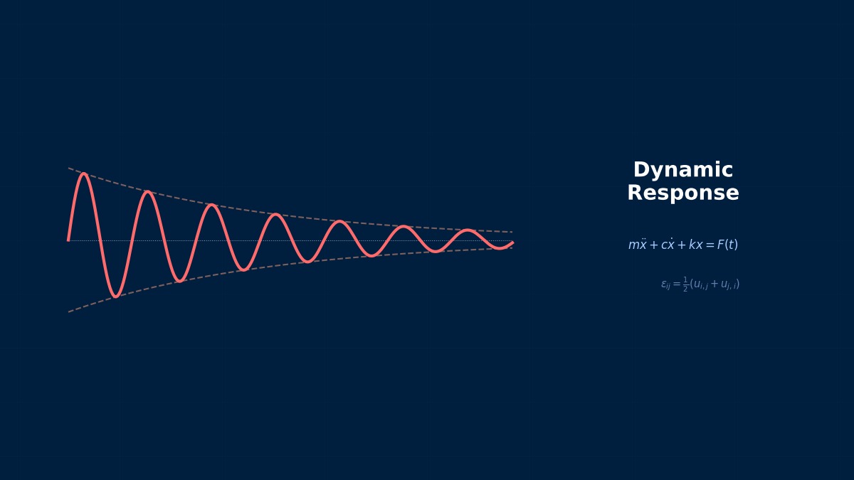

Equation of Motion

🎓

Earthquake input as base excitation:


$$ [M]\{\ddot{u}\} + [C]\{\dot{u}\} + [K]\{u\} = -[M]\{1\} \ddot{u}_g(t) $$

$\ddot{u}_g(t)$ is the earthquake acceleration time history (seismic waveform). $\{u\}$ is the relative displacement to the base.


🧑‍🎓

So you input the seismic waveform directly.


🎓

As design seismic waveforms:

  • Recorded Waves — Actual recorded waves like El Centro (1940), Hyogo-ken Nanbu Earthquake (1995), etc.
  • Simulated Seismic Waves — Artificially generated to match a design response spectrum.
  • Site-Specific Waves — Generated at the ground surface through ground response analysis.

Linear vs. Nonlinear

🎓
MethodMaterialAnalysis MethodPosition in Design Codes
Elastic Time HistoryElasticModal Method or Direct MethodLevel 1 Earthquake
Elastoplastic Time HistoryElastoplasticDirect Method (Newmark Method)Level 2 Earthquake
🧑‍🎓

So elastoplastic analysis is necessary for Level 2 earthquakes (major earthquakes).


🎓

For Level 2 earthquakes (Hyogo-ken Nanbu Earthquake class), structures yield, making elastoplastic time history analysis essential to track plastic hinge formation, energy absorption, and residual deformation.


Summary

🎓

Key Points:


  • Calculate the complete time history of the response by directly inputting the seismic waveform.
  • $[M]\{\ddot{u}\} + [C]\{\dot{u}\} + [K]\{u\} = -[M]\ddot{u}_g$ — Base excitation.
  • Elastic time history uses modal method, elastoplastic uses direct method — Newmark/HHT-α.
  • Input recorded waves or simulated seismic waves — Specified by design codes.
  • Elastoplastic time history is mandatory for Level 2 earthquakes — Plastic deformation and energy absorption.

Coffee Break Yomoyama Talk

Seismic time history analysis became widespread with computerization in the 1970s

Seismic time history response analysis is considered to have been practically established with calculations using the CAL16 code with the 1940 El Centro earthquake wave (accelerometer record 0.319g) in 1971. Subsequently, following the 1978 Miyagi-ken-oki earthquake, the revision of the Japanese Building Standards Act (1981, New Seismic Design Code) mandated time history analysis for super high-rise building design for structures over 60m tall. Computer centers like NTT Data began providing batch processing calculation services.

Physical Meaning of Each Term
  • Inertia Term (Mass Term): $\rho \ddot{u}$, i.e., "mass × acceleration". Have you ever experienced being thrown forward when slamming on the brakes? That "feeling of being carried away" is precisely the inertial force. Heavier objects are harder to set in motion and harder to stop once moving. Buildings shake during earthquakes because the ground moves suddenly while the building's mass "gets left behind". In static analysis, this term is set to zero, assuming "forces are applied slowly enough that acceleration can be ignored". It absolutely cannot be omitted for impact loads or vibration problems.
  • Stiffness Term (Elastic Restoring Force): $Ku$ or $\nabla \cdot \sigma$. When you stretch a spring, you feel a force "trying to return it", right? That's Hooke's law $F=kx$, the essence of the stiffness term. So a question—if you pull an iron rod and a rubber band with the same force, which stretches more? Obviously the rubber. This "resistance to stretching" is the Young's modulus $E$, which determines stiffness. A common misconception: "high stiffness = strong" is incorrect. Stiffness is "resistance to deformation", strength is "resistance to failure"—different concepts.
  • External Force Term (Load Term): Body force $f_b$ (gravity, etc.) and surface force $f_s$ (pressure, contact force, etc.). Think of it this way—the weight of a truck on a bridge is a force "acting on the entire volume" (body force), while the force of the tires pushing on the road surface is a force "acting only on the surface" (surface force). Wind pressure, water pressure, bolt tightening force... all are external forces. A common pitfall here: getting the load direction wrong. Intending "tension" but it becomes "compression"—sounds like a joke, but it actually happens when coordinate systems are rotated in 3D space.
  • Damping Term: Rayleigh damping $C\dot{u} = (\alpha M + \beta K)\dot{u}$. Try plucking a guitar string. Does the sound continue forever? No, it gradually fades. That's because vibrational energy is converted to heat by air resistance and internal friction in the string. Car shock absorbers work on the same principle—they intentionally absorb vibrational energy to improve ride comfort. What if damping were zero? Buildings would continue shaking forever after an earthquake. Since that doesn't happen in reality, setting appropriate damping is crucial.
Assumptions and Applicability Limits
  • Continuum assumption: Treats material as a continuous medium, ignoring microscopic heterogeneity.
  • Small deformation assumption (for linear analysis): Deformation is sufficiently small compared to initial dimensions, and the stress-strain relationship is linear.
  • Isotropic material (unless otherwise specified): Material properties are independent of direction (anisotropic materials require separate tensor definitions).
  • Quasi-static assumption (for static analysis): Ignores inertial and damping forces, considering only the balance between external and internal forces.
  • Non-applicable cases: Large deformation/large rotation problems require geometric nonlinearity. Nonlinear material behavior like plasticity and creep requires constitutive law extensions.
Dimensional Analysis and Unit Systems
VariableSI UnitNotes / Conversion Memo
Displacement $u$m (meter)When inputting in mm, unify loads and elastic modulus to MPa/N system.
Stress $\sigma$Pa (Pascal) = N/m²MPa = 10⁶ Pa. Be careful of unit inconsistency when comparing with yield stress.
Strain $\varepsilon$Dimensionless (m/m)Note the distinction between engineering strain and logarithmic strain (for large deformation).
Elastic Modulus $E$PaSteel: ~210 GPa, Aluminum: ~70 GPa. Note temperature dependence.
Density $\rho$kg/m³In mm system: tonne/mm³ (= 10⁻⁹ tonne/mm³ for steel).
Force $F$N (Newton)Unify as N in mm system, N in m system.

Numerical Methods and Implementation

Inputting Seismic Waveforms

🧑‍🎓

How do you input seismic waveforms into FEM?


Nastran

```

SOL 109 $ Direct method time history

CEND

DLOAD = 100

BEGIN BULK

TLOAD1, 100, 200, , 0, 300

TABLED1, 300, , ,

, 0.0, 0.0, 0.01, 1.23, 0.02, -0.56, ... $ Acceleration time history

```

Define acceleration with a TABLED1 table and apply it to the base SPC point.

Abaqus

```

*AMPLITUDE, NAME=earthquake

0.0, 0.0

0.01, 1.23

0.02, -0.56

...

*STEP

*DYNAMIC

0.01, 40.0 $ dt=0.01s, 40 seconds

*BASE MOTION, DOF=1, AMPLITUDE=earthquake

*END STEP

```

Ansys

```

/SOLU

ANTYPE, TRANSIENT

DELTIM, 0.01

TIME, 40.0

ACEL, , 9.81*amp(t) ! Acceleration input

SOLVE

```

🧑‍🎓

Abaqus's *BASE MOTION seems the simplest.


🎓

*BASE MOTION directly defines base excitation. You only specify the direction (DOF) and waveform (AMPLITUDE).


Elastoplastic Models

🎓

Material/element models used in seismic elastoplastic analysis:


Structure TypeModelFeatures
RC ColumnFiber Model (OpenSees)Tracks section plastification.
Steel BeamPlastic Hinge (Lumped Plasticity)Hinge element at ends.
Seismic Isolation DeviceBilinear SpringYield force and secondary stiffness.
Viscous DamperMaxwell ModelViscous + Elastic.

Summary

🎓
  • Abaqus *BASE MOTION is the simplest input — Specify direction and waveform.
  • Choose elastoplastic model according to structure type — RC: Fiber, Steel: Hinge.
  • $\Delta t = 0.005 \sim 0.01$ s is standard for seismic response — Covers up to 30 Hz.

  • Coffee Break Yomoyama Talk

    Japan's review criteria require averaging over 3 seismic waves

    For structural review of super high-rise buildings in Japan, Notification No. 457 requires that "the average of three or more waves (notification wave, site-specific wave, recorded wave) must keep each response value within the target value." Analysis methods are direct integration (Newmark-β, HHT-α) or mode superposition. For nonlinear analysis, trilinear or slip-type restoring force characteristics are adopted. The cost for one time history analysis run is about 30 minutes to 2 hours for a super high-rise building (~100 stories, ~30k DOF).

    Linear Elements (1st Order Elements)

    Linear interpolation between nodes. Low computational cost but low stress accuracy. Beware of shear locking (mitigated with reduced integration or B-bar method).

    Quadratic Elements (with Mid-Side Nodes)

    Can represent curved deformation. Stress accuracy improves significantly, but DOFs increase by about 2-3 times. Recommended when stress evaluation is important.

    Full Integration vs Reduced Integration

    Full Integration: Risk of over-constraint (locking). Reduced Integration: Risk of hourglass modes (zero-energy modes). Choose appropriately.

    Adaptive Mesh

    Automatic refinement based on error indicators (e.g., ZZ estimator). Efficiently improves accuracy in stress concentration areas. Includes h-method (element subdivision) and p-method (order increase).

    Newton-Raphson Method

    Standard method for nonlinear analysis. Updates the tangent stiffness matrix every iteration. Provides quadratic convergence within the convergence radius, but computational cost is high.

    Modified Newton-Raphson Method

    Updates the tangent stiffness matrix using the initial value or every few iterations. Cost per iteration is low, but convergence speed is linear.

    Convergence Criteria

    Force residual norm: $||R|| / ||F_{ext}|| < \epsilon$ (typically $\epsilon = 10^{-3}$〜$10^{-6}$). Displacement increment norm: $||\Delta u|| / ||u|| < \epsilon$. Energy norm: $\Delta u \cdot R < \epsilon$

    Load Increment Method

    Applies the full load not all at once, but in small increments. The arc-length method (Riks method) can trace beyond limit points on the load-displacement curve.

    Analogy for Direct vs. Iterative Methods

    The direct method is like "solving simultaneous equations accurately with pen and paper"—reliable but too time-consuming for large-scale problems. The iterative method is like "repeatedly guessing to approach the correct answer"—starts with a rough answer but improves accuracy with each iteration. It's the same principle as looking up a word in a dictionary: it's more efficient to open it at an estimated location and adjust forward/backward (iterative) than to search sequentially from the first page (direct).

    Relationship Between Mesh Order and Accuracy

    1st order elements are like "approximating a curve with a ruler"—represented by straight line segments, so accuracy is limited. 2nd order elements are like a "flexible curve"—can represent curved changes, dramatically improving accuracy even at the same mesh density. However, computational cost per element increases, so judge based on total cost-effectiveness.

    Practical Guide

    Seismic Time History in Practice

    🎓

    Used in the Building Standards Act's "Limit Strength Calculation Method" and "Time History Response Analysis".


    Seismic Waveform Selection

    🎓

    Seismic waves specified by design codes:


    CodeSeismic Wave Selection
    Japan (Notification)3 or more recorded waves + site-specific waves. Extremely rare ground motions.
    Eurocode 8Simulated seismic waves compatible with response spectrum. Minimum 3 waves.
    ASCE 77 or more waves. Spectrum compatible with ground characteristics.
    NRC (Nuclear)SSE (Safe Shutdown Earthquake) compatible waves. Probabilistic hazard.
    🧑‍🎓

    So you analyze with a minimum of 3 seismic waves.


    🎓

    Average over 3 waves, use the maximum value from each of 7 waves (ASCE 7). The basic principle is to evaluate result variability with multiple seismic waves.


    Result Evaluation

    関連シミュレーター

    この分野のインタラクティブシミュレーターで理論を体感しよう

    シミュレーター一覧

    関連する分野

    熱解析製造プロセス解析V&V・品質保証
    この記事の評価
    ご回答ありがとうございます!
    参考に
    なった
    もっと
    詳しく
    誤りを
    報告
    参考になった
    0
    もっと詳しく
    0
    誤りを報告
    0
    Written by NovaSolver Contributors
    Anonymous Engineers & AI — サイトマップ
    About the Authors