Augmented Lagrangian法
Theory and Physics
What is the Augmented Lagrangian Method?
Professor, is the Augmented Lagrangian method a "best of both worlds" combination of the Penalty method and the Lagrange multiplier method?
Exactly. It's a technique that combines the simplicity of the Penalty method with the zero-penetration accuracy of the Lagrange multiplier method.
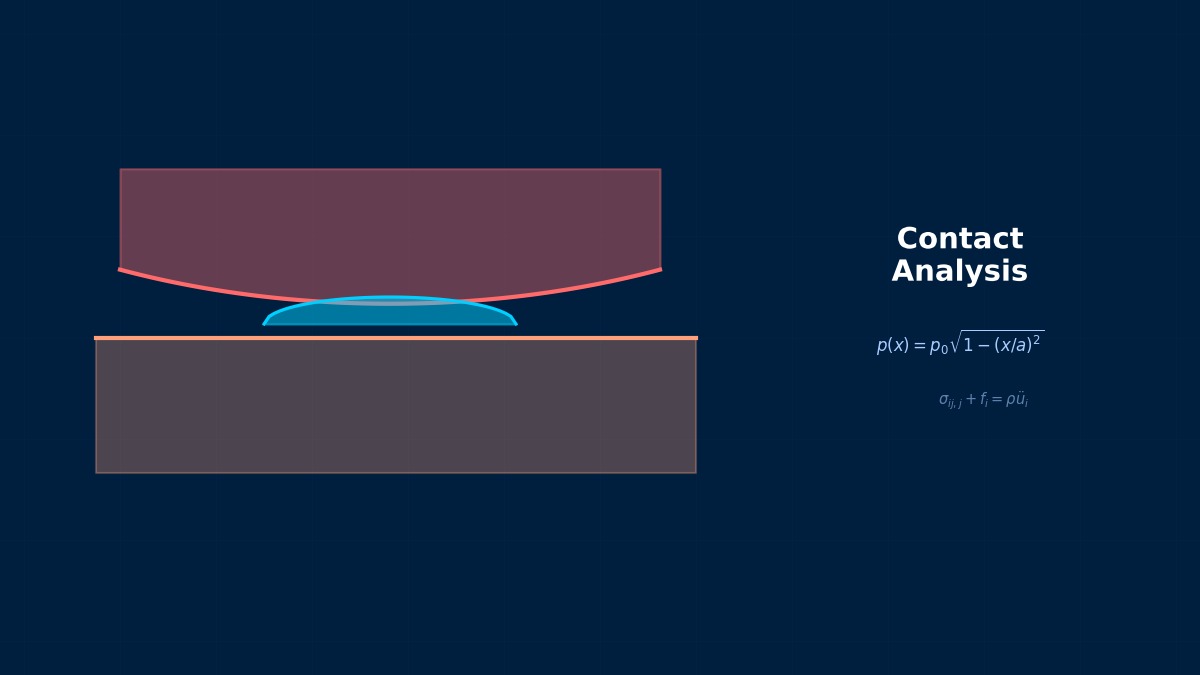
In addition to the penalty term $k_p g_n$, the Lagrange multiplier $\lambda_n$ is iteratively updated. As iterations proceed, penetration converges to zero.
So even with a small penalty stiffness $k_p$, penetration can be reduced through iteration, right?
Its dependence on $k_p$ is smaller than the Penalty method. This is its greatest advantage. Augmented Lagrangian is the default in Ansys.
Summary
Key Points:
- Penalty + Iterative Lagrange Update — Best of both worlds
- Small dependence on $k_p$ — More stable than the Penalty method
- No additional DOFs required — More efficient than the Lagrange multiplier method
- Ansys Default — The most widely recommended method
Hestenes-Powell Method 1969
The Augmented Lagrangian method is a hybrid technique combining penalty and Lagrange multipliers, independently published by M.R. Hestenes and M.J.D. Powell in 1969. By updating the multipliers with each outer iteration, it avoids the ill-conditioning of pure penalty methods while also avoiding the large-scale simultaneous equations of pure multiplier methods. Its application to contact FEM was systematized by Simo and Laursen in the late 1980s.
Physical Meaning of Each Term
- Inertia Term (Mass Term): $\rho \ddot{u}$, meaning "mass × acceleration". Have you ever experienced being thrown forward when slamming on the brakes? That "feeling of being carried away" is precisely the inertial force. Heavier objects are harder to set in motion and harder to stop once moving. Buildings shake during earthquakes because the ground moves suddenly while the building's mass "gets left behind". In static analysis, this term is set to zero, based on the assumption that "forces are applied slowly enough that acceleration can be ignored". It absolutely cannot be omitted for impact loads or vibration problems.
- Stiffness Term (Elastic Restoring Force): $Ku$ or $\nabla \cdot \sigma$. When you stretch a spring, you feel a "force trying to return it", right? That's Hooke's law $F=kx$, the essence of the stiffness term. Now a question — an iron rod and a rubber band, which stretches more under the same force? Obviously the rubber. This "resistance to stretching" is the Young's modulus $E$, which determines stiffness. A common misconception: "high stiffness = strong" is incorrect. Stiffness is "resistance to deformation", strength is "resistance to failure" — they are different concepts.
- External Force Term (Load Term): Body forces $f_b$ (gravity, etc.) and surface forces $f_s$ (pressure, contact forces, etc.). Think of it this way — the weight of a truck on a bridge is a "force acting on the entire volume" (body force), while the force of the tires pushing on the road surface is a "force acting only on the surface" (surface force). Wind pressure, water pressure, bolt tightening force... all are external forces. A common pitfall here: getting the load direction wrong. Intending "tension" but modeling "compression" — sounds like a joke, but it actually happens when coordinate systems are rotated in 3D space.
- Damping Term: Rayleigh damping $C\dot{u} = (\alpha M + \beta K)\dot{u}$. Try plucking a guitar string. Does the sound continue forever? No, it gradually fades away. That's because vibrational energy is converted to heat by air resistance and internal friction in the string. Car shock absorbers work on the same principle — intentionally absorbing vibrational energy to improve ride comfort. What if damping were zero? Buildings would continue swaying forever after an earthquake. Since that doesn't happen in reality, setting appropriate damping is crucial.
Assumptions and Applicability Limits
- Continuum Assumption: Treats material as a continuous medium, ignoring microscopic heterogeneity.
- Small Deformation Assumption (for linear analysis): Deformation is sufficiently small compared to initial dimensions, and the stress-strain relationship is linear.
- Isotropic Material (unless otherwise specified): Material properties are independent of direction (anisotropic materials require separate tensor definitions).
- Quasi-Static Assumption (for static analysis): Ignores inertial and damping forces, considering only the balance between external and internal forces.
- Non-Applicable Cases: For large deformation/large rotation problems, geometric nonlinearity is required. For nonlinear material behavior like plasticity or creep, constitutive law extensions are needed.
Dimensional Analysis and Unit Systems
| Variable | SI Unit | Notes / Conversion Memo |
|---|---|---|
| Displacement $u$ | m (meter) | When inputting in mm, unify loads and elastic modulus to MPa/N system. |
| Stress $\sigma$ | Pa (Pascal) = N/m² | MPa = 10⁶ Pa. Be careful of unit inconsistency when comparing with yield stress. |
| Strain $\varepsilon$ | Dimensionless (m/m) | Note the distinction between engineering strain and logarithmic strain (for large deformations). |
| Elastic Modulus $E$ | Pa | Steel: ~210 GPa, Aluminum: ~70 GPa. Note temperature dependence. |
| Density $\rho$ | kg/m³ | In mm system: tonne/mm³ (= 10⁻⁹ tonne/mm³ for steel). |
| Force $F$ | N (Newton) | Unify to N in mm system, N in m system. |
Numerical Methods and Implementation
Implementation of Augmented Lagrangian
Algorithm:
1. Solve initially as a Penalty method with $\lambda = 0$
2. Check penetration amount $g_n$
3. Update $\lambda$: $\lambda \leftarrow \lambda + k_p g_n$
4. Solve again with the updated $\lambda$
5. Iterate until $g_n$ becomes sufficiently small
So there's an outer loop ($\lambda$ update) and an inner loop (Newton-Raphson), right?
A double iteration loop. The inner loop satisfies equilibrium, the outer loop satisfies contact constraints. Computational cost is about 1.5 to 2 times that of the Penalty method.
Solver Settings
Summary
Multiplier Update Iteration Scheme
Augmented Lagrangian contact has a double iteration structure: an outer loop updates the Lagrange multiplier λ, and an inner loop solves the nonlinear finite element solution. In the formulation by Laursen & Simho (1993), the multiplier update formula λ_{k+1} = λ_k + ε_N g_N (g_N: penetration, ε_N: penalty) is adopted. Since ε_N can be set intuitively by back-calculating from physical gap tolerance, convergence tuning is more intuitive than with the Penalty method.
Linear Elements (1st Order Elements)
Linear interpolation between nodes. Computational cost is low, but stress accuracy is low. Beware of shear locking (mitigated by reduced integration or B-bar method).
Quadratic Elements (with Midside Nodes)
Can represent curved deformation. Stress accuracy improves significantly, but degrees of freedom increase by about 2~3 times. Recommendation: When stress evaluation is important.
Full Integration vs Reduced Integration
Full Integration: Risk of over-constraint (locking). Reduced Integration: Risk of hourglass modes (zero-energy modes). Choose appropriately for the situation.
Adaptive Mesh
Automatic refinement based on error indicators (e.g., ZZ estimator). Efficiently improves accuracy in stress concentration areas. Includes h-method (element subdivision) and p-method (order increase).
Newton-Raphson Method
Standard method for nonlinear analysis. Updates the tangent stiffness matrix each iteration. Achieves quadratic convergence within the convergence radius, but computational cost is high.
Modified Newton-Raphson Method
Updates the tangent stiffness matrix using the initial value or every few iterations. Cost per iteration is low, but convergence speed is linear.
Convergence Criteria
Force residual norm: $||R|| / ||F_{ext}|| < \epsilon$ (typically $\epsilon = 10^{-3}$ to $10^{-6}$). Displacement increment norm: $||\Delta u|| / ||u|| < \epsilon$. Energy norm: $\Delta u \cdot R < \epsilon$
Load Increment Method
Instead of applying the full load at once, apply it in small increments. The arc-length method (Riks method) can track beyond limit points on the load-displacement curve.
Analogy: Direct Method vs Iterative Method
The direct method is like "solving simultaneous equations accurately with pen and paper" — reliable but takes too long for large-scale problems. The iterative method is like "repeatedly guessing to approach the correct answer" — starts with a rough answer but improves accuracy with each iteration. It's the same principle as looking up a word in a dictionary: opening to an estimated page and adjusting forward/backward (iterative) is more efficient than searching sequentially from the first page (direct).
Relationship Between Mesh Order and Accuracy
1st order elements are like "approximating a curve with a ruler" — represented by straight line segments, so accuracy is limited. 2nd order elements are like "flexible curves" — can represent curved changes, dramatically improving accuracy even at the same mesh density. However, computational cost per element increases, so judgment should be based on total cost-effectiveness.
Practical Guide
Augmented Lagrangian in Practice
Many Ansys users unconsciously use Augmented Lagrangian. The default is the most stable.
Practical Checklist
Aircraft Engine Blade Fretting
Around 2008, GE Aviation began using ANSYS Mechanical's Augmented Lagrangian contact to analyze fretting wear in turbine blade dovetail sections. They evaluated repeated contact equivalent to 10⁷ cycles combined with a cumulative damage model, reproducing wear depth on Inconel 718 blades with an accuracy of ±15μm compared to measured values. This case was presented at an academic conference as an example that reduced prototype manufacturing costs by about 30%.
Analogy of the Analysis Flow
The analysis flow is actually very similar to cooking. First, you buy ingredients (prepare the CAD model), do the prep work (mesh generation), apply heat (solver execution), and finally plate it (visualization in post-processing). Here's an important question — in cooking, which step is most prone to failure? Actually, it's the "prep work". If mesh quality is poor, the results will be a mess no matter how excellent the solver is.
Pitfalls Beginners Easily Fall Into
Are you checking mesh convergence? Do you think "the calculation ran = the result is correct"? This is actually the most common trap for CAE beginners. The solver will always return "some answer" for the given mesh. But if the mesh is too coarse, that answer will be far from reality. Confirm that results stabilize across at least three levels of mesh density — neglecting this leads to the dangerous assumption that "the computer gave the answer, so it must be correct".
Thinking About Boundary Conditions
Setting boundary conditions is the same as "writing the problem statement" for an exam. If the problem statement is wrong? No matter how accurately you calculate, the answer will be wrong. "Is this surface truly fully fixed?" "Is this load truly uniformly distributed?" — Correctly modeling real-world constraint conditions is actually the most critical step in the entire analysis.
Software Comparison
Tools for Augmented Lagrangian
Selection Guide
Evolution of ANSYS ALM Implementation
ANSYS adopted the Augmented Lagrange Method (ALM) as the default contact algorithm for CONTA174/TARGE170 elements in the late 1990s. In ANSYS 10.0 (2005), the ALM convergence criterion was revised to a contact force basis, significantly improving penetration issues in thick plates. In the current ANSYS Mechanical 2024, the "program controlled" setting, which automatically switches between ALM and the Penalty method, is the default.
The Three Most Important Questions for Selection
- "What are you solving?": Does the required physical model/element type support the Augmented Lagrangian method? For example, in fluids, the presence of LES support; in structures, the ability to handle contact/large deformation makes a difference.
- "Who will use it?": For beginner teams, tools with rich GUIs are suitable; for experienced users, flexible script-driven tools are better. Similar to the difference between an automatic transmission car (GUI) and a manual transmission car (script).
- "How far will it expand?": Selection considering future analysis scale expansion (HPC support), deployment to other departments, and integration with other tools leads to long-term cost reduction.
Advanced Technology
Advanced Topics in Augmented Lagrangian
Related Topics
なった
詳しく
報告