Penalty Method-Based Contact Formulation
Penalty Method-Based Contact Formulation: Theoretical Foundations
Fundamentals of Contact Problems
Professor, what makes FEM "contact problems" so difficult?
Contact problems are inherently nonlinear. There are three reasons:
1. State Change — The contact surface has a binary state of "Contact/No Contact". The state changes with load.
2. Inequality Constraint — Penetration must not occur: $g \geq 0$
3. Friction — Coulomb friction involves state changes between "stick/slip".
Inequality constraints... That's fundamentally different from the equality constraints (like SPC) in regular FEM.
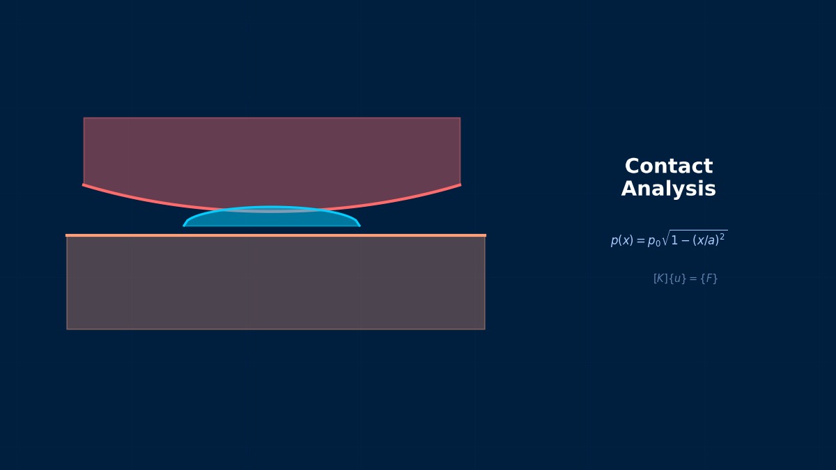
Regular FEM solves the equality $[K]\{u\} = \{F\}$, but contact must satisfy the KKT conditions (Karush-Kuhn-Tucker conditions): "$g \geq 0$ and $g \cdot p = 0$". $g$ is the gap, $p$ is the contact pressure.
Principle of the Penalty Method
The Penalty Method is the simplest contact handling technique. It adds a "reaction force proportional to penetration":
$k_p$ is the penalty stiffness (contact stiffness). $g_n$ is the normal penetration amount.
It's like putting a spring at the contact surface.
Exactly. The penalty method places a very stiff spring at the contact surface. When penetration occurs, a reaction force is generated, pushing back the penetration.
Setting Penalty Stiffness
The setting of penalty stiffness $k_p$ greatly influences the results:
- $k_p$ too large → Condition number worsens. Convergence becomes difficult.
- $k_p$ too small → Penetration amount becomes excessive. Inaccurate.
Guideline: $k_p \approx 10 \sim 100 \times E \cdot A / L$ (on the order of the contact surface stiffness). Many solvers calculate this automatically.
Is it safe to rely on automatic calculation?
For most cases, yes. The automatic penalty stiffness in Abaqus or Ansys is a good starting point. Only adjust manually when problems arise.
Advantages and Disadvantages of the Penalty Method
| Advantages | Disadvantages |
|---|---|
| Simple implementation | Penetration does not become exactly zero |
| No additional DOFs required | Penalty stiffness setting affects results |
| Compatible with explicit methods | Large $k_p$ worsens condition number |
| Default for many solvers | — |
Is "penetration not becoming zero" the biggest weakness?
As long as $k_p$ is finite, slight penetration is unavoidable. If the penetration amount is less than 1% of the plate thickness, it's practically acceptable. If more, consider the Lagrange multiplier method.
Summary
Key Points:
- Contact is a nonlinear problem with inequality constraints — State change + Friction
- Penalty Method = Spring at contact surface — $F = k_p \cdot g_n$
- $k_p$ setting is key — Too large causes convergence difficulty, too small causes excessive penetration
- Many solvers calculate automatically — Manual adjustment only when problems occur
- Penetration does not become exactly zero — Aim for less than 1% of plate thickness
Courant's 1943 Penalty Method
The mathematical origin of the penalty method lies in Richard Courant's 1943 paper "Variational methods for the solution of problems of equilibrium and vibrations". The idea of transforming a constrained variational problem into an unconstrained one by adding a term multiplied by a large coefficient (penalty) was initially used for handling boundary conditions of elliptic partial differential equations. In the 1970s, Oden & Kim (1977) and others systematically applied it to contact FEM.
Computational Methods for Penalty Method-Based Contact Formulation
Implementation of the Penalty Method
How is the penalty method set up in each solver?
Abaqus
```
*CONTACT PAIR, INTERACTION=contact_prop
slave_surface, master_surface
*SURFACE INTERACTION, NAME=contact_prop
*SURFACE BEHAVIOR, PENALTY
```
Abaqus default is the penalty method. Specify explicitly with *SURFACE BEHAVIOR, PENALTY.
Nastran
```
BCTABLE, ...
BCPARA, CTYPE, UGLYPEN $ Penalty Method
```
Contact definition in Nastran SOL 101/106/400.
Ansys
```
MP, MU, cid, 0.3 ! Friction coefficient
KEYOPT, cid, 2, 1 ! Penalty Method
```
Or in Workbench Contact settings, Formulation=Penalty.
LS-DYNA
```
*CONTACT_AUTOMATIC_SURFACE_TO_SURFACE
$ Penalty method is default
```
All LS-DYNA contacts are penalty method based. The most natural method for explicit analysis.
Contact Detection
Penalty method procedure (each iteration):
1. Contact Detection — Search for the closest point of slave nodes on the master surface.
2. Gap Calculation — $g_n$ = distance between slave node and master surface.
3. Penetration Judgment — If $g_n < 0$, contact. Reaction force $F_n = k_p |g_n|$.
4. Friction Force Calculation — $F_t = \mu F_n$ (slip) or stick.
5. Reflect in Global Equation — Add penalty force to the right-hand side.
Does contact detection account for most of the computational cost?
For large-scale models (hundreds of thousands of contact element pairs), contact detection can account for 30-50% of computation time. Fast search algorithms like Bucket sort and KD-tree are used.
Summary
- Penalty method is default in all major solvers — Setup is simple.
- Contact detection → Gap calculation → Reaction force → Global equation — Executed each iteration.
- Contact detection is 30-50% of computation — Bottleneck for large-scale contact.
- All LS-DYNA contacts are penalty method — Best compatibility with explicit methods.
Selection Rule for Penalty Stiffness
Choosing the contact penalty coefficient ε is the most important practical issue in the penalty method. If ε is too small, penetration exceeds allowable values; if too large, the condition number of the stiffness matrix worsens and convergence slows. LS-DYNA's default setting uses the "SOFT=0" algorithm which automatically sets ε to 0.1 times the minimum element stiffness k_e (=E×t×A) of the contact surface. For dissimilar material contact (e.g., steel-resin), manual tuning is recommended.