Place up to 3 point charges freely and watch the electric field arrows and potential color map update in real time via Coulomb superposition. Equipotential contours and a V(x) cross-section chart included.
Point Charges
Charge 1 (+)
q₁
μC
x₁
m
y₁
m
Charge 2 (−)
q₂
μC
x₂
m
y₂
m
Charge 3 (+)
q₃
μC
x₃
m
y₃
m
Cursor Readout
While paused, move the sliders to update the result instantly.
Live Probe Readout
— kV
Potential V
— kV/m
Field |E|
— pN
Force on +1 nC
— m
Nearest charge dist.
Field Lines & Flow (animated)
Particles stream along the field lines — out of positive charges and into negative charges. Move the cursor over the canvas to set the probe point and read potential and field strength.
What exactly is the difference between the electric field and the electric potential? The simulator shows arrows and colored contours, but I'm not sure what each one is telling me.
🎓
Great question! Basically, think of the electric field as a "force field" and the potential as an "energy landscape." The arrows you see show the direction and strength of the force a tiny positive test charge would feel. The colored contours, called equipotential lines, connect points with the same potential energy per charge. In practice, a positive charge will always try to "roll downhill" from high to low potential. Try placing a single positive charge in the simulator and watch how the arrows point away from it, while the potential contours form circles around it.
🙋
Wait, really? So the field arrows are perpendicular to those colored contour lines? That seems like a weird coincidence.
🎓
It's not a coincidence—it's a fundamental rule! The electric field vector at any point is always perpendicular to the equipotential line and points in the direction of decreasing potential. This is captured by the relation $\vec{E}=-\nabla V$. For instance, in the simulator, drag two positive charges close together. You'll see the field arrows push away from the "hill" created by the charges, and they are always perpendicular to the tightly packed contour lines in between them.
🙋
That makes sense. So when I add a third charge with the parameter controls, the whole pattern changes. How does the math handle that? Is it just adding everything up?
🎓
Exactly! That's the superpower of the principle of superposition. The total electric field or potential at any point is simply the vector or scalar sum, respectively, of the contributions from each individual point charge. This is why the simulator can update in real-time as you move the sliders for q₃, x₃, y₃. A common case is designing a capacitor: engineers place opposite charges to create a nearly uniform field in between. Try setting q₁ = +1, q₂ = -1 and aligning them horizontally to see this classic pattern emerge.
Physical Model & Key Equations
The electric field $\vec{E}$ at a point in space due to a collection of point charges is the vector sum of the fields from each charge. The strength from a single charge drops with the square of the distance.
$$\vec{E}=\sum_i k\frac{q_i}{r_i^2}\hat{r}_i$$
Here, $k$ is Coulomb's constant ($8.99 \times 10^9\ \mathrm{N \cdot m^2/C^2}$), $q_i$ is the value of the i-th charge, $r_i$ is the distance from the charge to the point, and $\hat{r}_i$ is a unit vector pointing from the charge to the point. A positive charge creates a field pointing away from it.
The electric potential $V$ is a scalar quantity representing the potential energy per unit charge. It is much easier to calculate than the vector field because we just add numbers, not directions.
$$V=\sum_i k\frac{q_i}{r_i}$$
The potential from a single charge falls off as $1/r$, not $1/r^2$. The key relationship is $\vec{E}=-\nabla V$, meaning the electric field is the negative gradient (steepest downhill slope) of the potential. This is why field lines are perpendicular to equipotential contours.
Frequently Asked Questions
This simulator is designed for real-time updates by default, but updates may be paused to reduce browser load. Please check the 'Update' button or 'Auto Update' toggle on the screen and enable it. If it still does not update, try reloading the page.
The potential color map visualizes the potential at each point on the plane using color gradients (blue for low potential, red for high potential). Equipotential lines connect points with the same potential, and denser lines indicate a stronger electric field. Using both together allows you to grasp the overall potential distribution and details simultaneously.
k is fixed as a physical constant in a vacuum (8.99×10^9) to align with real-world electromagnetism. However, if you only need relative comparisons for educational purposes, you can input charge amounts as arbitrary relative values (e.g., +1, -2).
Yes, you can zoom in and out using the mouse wheel and pan the screen by dragging. Additionally, pressing the 'Reset Display Range' button in the control panel on the right will automatically adjust the view to fit all point charges optimally.
Real-World Applications
Semiconductor Device Design: Engineers use these exact calculations to model how electric fields and potentials shape the "electron landscape" inside transistors and microchips. By simulating the placement of charge regions (doping), they can control the flow of current.
Electrostatic Precipitators: Used in power plants and factories to clean air. Charged plates create a strong, non-uniform electric field (like in the simulator with two opposite charges). Soot particles become charged and are pulled by the field onto the plates, removing them from the exhaust stream.
Medical Equipment (CRT Monitors & X-ray Tubes): Old cathode-ray tube (CRT) TVs and monitors used precisely shaped electric fields to steer a beam of electrons to paint an image on the screen. Similarly, X-ray tubes use high potentials to accelerate electrons to extreme speeds.
Geophysical Exploration: Scientists measure subtle variations in the electric potential at the Earth's surface to map underground structures. Different rock and fluid layers create distortions in the field, helping to locate aquifers, mineral deposits, or archaeological sites.
Common Misconceptions and Points to Note
When you start using this simulator, there are a few points you should be aware of. First, you might tend to think that "the length of the electric field vector is proportional to the electric potential at that location," but that is a misconception. The strength of the electric field is determined by the "steepness of the potential gradient," i.e., the rate of change. For example, on a flat, high-potential plateau (where equipotential lines are widely spaced) the electric field is weak, whereas in a steep, low-potential valley (where equipotential lines are dense) the electric field is strong. Try verifying this on the screen.
Next, while point charges can be placed infinitely close in the simulator, in practice, there is a defined range within which they can be treated as "points." For instance, if a 1 mm² electrode carries a charge of 1 nC, it can be considered almost a point charge at distances greater than a few centimeters away. However, within 1 mm of the electrode surface, you need to consider the charge distribution. This sense of scale is crucial when directly applying the tool's results to real-world situations.
Finally, remember that the superposition principle, which is fundamental to this simulator's calculations, holds true only in linear media (roughly, vacuum or air). If strongly polarizing materials (ferroelectrics) or conductors are present nearby, the field becomes significantly distorted by the induced charges they create, making it impossible to calculate by simple addition. Understand that this is a simulation in an "idealized environment" for learning fundamental principles.
Enter the number of point charges (en1) and their magnitudes in microcoulombs (q1, q2, etc.) using the input fields
Set spatial coordinates (x1num, y1num) in meters for each charge position on the 2D grid
Click "Simulate" to generate real-time field vectors and equipotential contours; observe potential V in volts and field magnitude |E| in V/m at any probe location
Adjust charge values or positions dynamically to see immediate updates in field topology
Worked Example
Place +1 μC at (-0.5 m, 0) and -1 μC at (+0.5 m, 0). At the grid midpoint (0, 0), the potential is V=0 V and the electric-field magnitude is |E|=7.19×10⁴ V/m, directed from the positive charge toward the negative charge (+x direction). At the outside grid point (1.5 m, 0), the distances are 1.0 m to the negative charge and 2.0 m to the positive charge, giving V≈-4.50×10³ V and |E|≈6.74×10³ V/m directed leftward toward the negative charge.
Practical Notes
Use small charge magnitudes (under 10 µC) to avoid numerical instability in field calculations near singularities
Space charges at least 0.05 m apart to prevent solver artifacts; converge at ~0.01 m grid resolution
Opposite charges create dipole moments useful for modeling molecular electrostatics in organic compounds
Same-polarity charges demonstrate Coulomb repulsion force proportional to q₁q₂/r² for capacitor plate design verification
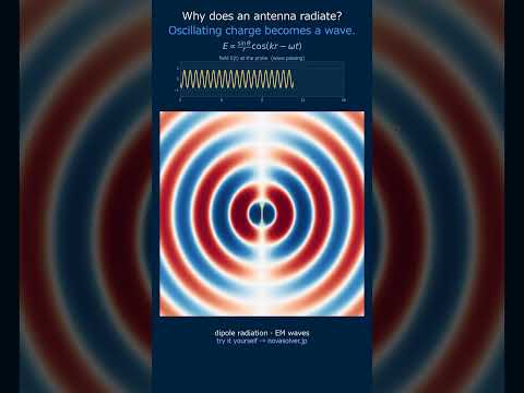
🎬 Watch it in motion
Electric Dipole | the field two opposite charges weave #Shorts