Visualize the potential distribution from multiple point charges on a red-blue color map. Draw equipotential lines and electric field vectors in real time to explore dipoles, repulsive charges, and multipole structures.
Charge Settings
nC
nC
nC
m
Test charge rolling down the potential landscape (live)
A positive test charge rolls perpendicular to the equipotential lines, from high to low potential (E = -∇V).
Results (live)
Potential V at test charge
—V
|E| at test charge
—V/m
Potential energy U of test charge
—nJ
Potential at Midpoint
—V
Potential at Charge 1 Position
—V
Field at midpoint
—V/m
Total q₁+q₂+q₃
—nC
Pot
Negative (blue)Positive (red)
Field
Cross
Theory & Key Formulas
$V = k\sum_i \dfrac{q_i}{r_i}$
$k = 9\times10^9\ \mathrm{N\cdot m^2/C^2}$
Relationship between electric field and potential:
💬 Electric Field and Potential — Reading the Topographic Map of 'Invisible Forces'
🙋
What is electric potential? I learned that electric field is the direction of force, but what is potential the 'potential' of?
🎓
The easiest way to think of electric potential is as 'height'. Just as on a topographic map of a mountain, higher elevation means higher gravitational potential energy, a location with high electric potential means a positive charge has difficulty moving there (i.e., work is needed to bring it there). The electric field is the 'slope' of the potential: the steeper the mountain, the larger the gradient (slope), meaning a stronger electric field. Think of the red areas on the color map as 'mountain peaks' and the blue areas as 'valley floors'.
🙋
Equipotential lines are like contour lines, right? But why is the electric field vector always perpendicular to equipotential lines?
🎓
The electric field is $\mathbf{E} = -\nabla V$, i.e., the negative gradient of the potential. And the gradient vector is always perpendicular to contour lines (equipotential lines)—this is a fundamental property of differential geometry. When walking on a mountain, the steepest downhill direction is perpendicular to the contour lines, right? Similarly, electric field lines (direction of the electric field) are always orthogonal to equipotential lines.
🙋
The potential distribution of a dipole isn't symmetric, is it? The positive charge side is red, and the negative charge side is blue.
🎓
That's right. A dipole has +q and -q close together. Near +q, V > 0 (red); near -q, V < 0 (blue); on the perpendicular bisector of the line connecting them, V = 0. This V = 0 surface is at the center of the equipotential surfaces. Far away, the potential drops faster than 1/r—for a monopole it drops as 1/r, for a dipole as 1/r². That's the key point.
🙋
For like charges (+q and +q), there seems to be a special point in the middle, right?
🎓
That 'special point' is where the electric field is zero—called a 'saddle point'. At the midpoint between two positive charges, the Coulomb forces from each cancel out exactly, so the electric field $\mathbf{E} = 0$. But the potential is not zero (it's still positive at that point). The potential can be non-zero even when the electric field is zero—this means 'the gradient of the potential is zero = the potential is flat', corresponding to a mountain peak or a saddle (a low point between mountains).
🙋
Where is this knowledge used in actual engineering?
🎓
Potential calculations are used widely in capacitor design, electrostatic shielding, MRI magnet design, and more. In CAE (Computer-Aided Engineering), the finite element method (FEM) solves Poisson's equation $\nabla^2 V = -\rho/\varepsilon_0$ to obtain the potential distribution. When electric field 'concentration' occurs, there is a risk of dielectric breakdown (discharge), so checking the electric field distribution during design is fundamental in electrical engineering. For example, the 'edge effect' where the electric field suddenly increases at the edges of a capacitor can be intuitively understood using a two-charge model in this tool.
Frequently Asked Questions
What is the difference between electric potential and electric field?
Electric potential $V$ is a scalar quantity (unit: V) representing the work required to bring a unit positive charge from infinity. The electric field $\mathbf{E}$ is a vector quantity (unit: V/m) representing the direction and magnitude of the force on a positive charge. The relationship is $\mathbf{E} = -\nabla V$, with the electric field pointing from high to low potential. It is practical to compute the scalar potential first and then derive the vector electric field.
Why are equipotential lines and electric field lines orthogonal?
The electric field is the gradient of the potential ($\mathbf{E} = -\nabla V$). Mathematically, the gradient vector is perpendicular to contour lines (equipotential lines). Moving along an equipotential line results in no change in potential, so the rate of change in that direction is zero, meaning the electric field component is zero—this is equivalent to the electric field being perpendicular to the equipotential line. This has been verified experimentally and is one of the most fundamental properties of electromagnetism.
How does the distance dependence of potential differ between a dipole and a monopole?
For a monopole (single point charge), $V \propto 1/r$ (inverse of distance). For a dipole (+q and -q pair), the potential at a distance is $V \propto 1/r^2$ (inverse square of distance). This is because the positive and negative contributions partially cancel. For a quadrupole, it's $1/r^3$, and in general, a $2^n$-pole has $1/r^{n+1}$ dependence. As distance increases, the influence of a dipole decays more rapidly than that of a monopole.
Where is the point where the electric field is zero for two like charges?
For two positive charges $q_1$ and $q_2$ separated by distance $d$, the point where the electric field is zero lies on the line connecting them. Its position is $x = d \cdot \sqrt{q_1} / (\sqrt{q_1} + \sqrt{q_2})$ (distance from $q_1$). For equal charges, it is the midpoint. This point is also called an 'equilibrium point' where a test charge experiences no net force, but it is an unstable equilibrium (a slight displacement results in a large force).
Why is the finite element method necessary for electric field calculation in CAE?
Analytical solutions exist for point charges in vacuum, but real-world designs involve complex electrode shapes, dielectrics, and conductors. In such cases, the potential follows Poisson's equation $\nabla^2 V = -\rho/\varepsilon$, which is solved numerically using the finite element method (FEM). Typical tools include COMSOL Multiphysics and ANSYS Maxwell, which generate a mesh based on the geometry and perform the calculation.
What is Electric Potential Field Simulator?
Electric Potential Field Simulator is a fundamental topic in engineering and applied physics. This interactive simulator lets you explore the key behaviors and relationships by directly manipulating parameters and observing real-time results.
By combining numerical computation with visual feedback, the simulator bridges the gap between abstract theory and physical intuition — making it an effective learning tool for students and a rapid-verification tool for practicing engineers.
Physical Model & Key Equations
The simulator is based on the governing equations behind Electric Potential Field Simulator. Understanding these equations is key to interpreting the results correctly.
Each parameter in the equations corresponds to a slider in the control panel. Moving a slider changes the equation's solution in real time, helping you build a direct connection between mathematical expressions and physical behavior.
Real-World Applications
Engineering Design: The concepts behind Electric Potential Field Simulator are applied across mechanical, structural, electrical, and fluid engineering disciplines. This tool provides a quick way to estimate design parameters and sensitivity before committing to full CAE analysis.
Education & Research: Widely used in engineering curricula to connect theory with numerical computation. Also serves as a first-pass validation tool in research settings.
CAE Workflow Integration: Before running finite element (FEM) or computational fluid dynamics (CFD) simulations, engineers use simplified models like this to establish physical scale, identify dominant parameters, and define realistic boundary conditions.
Common Misconceptions and Points of Caution
Model assumptions: The mathematical model used here relies on simplifying assumptions such as linearity, homogeneity, and isotropy. Always verify that your real system satisfies these assumptions before applying results directly to design decisions.
Units and scale: Many calculation errors arise from unit conversion mistakes or order-of-magnitude errors. Pay close attention to the units shown next to each parameter input.
Validating results: Always sanity-check simulator output against physical intuition or hand calculations. If a result seems unexpected, review your input parameters or verify with an independent method.
Set the number of charges using sl_q1Num, sl_q2Num, and sl_q3Num (1-3 charges maximum)
Define charge magnitudes in coulombs via sl_q1, sl_q2, sl_q3 (range: -10 µC to +10 µC)
Adjust charge separation distance with sl_sep (0.1 m to 2 m spacing)
Click simulate to render the potential field color map and equipotential contours
Hover over the field to read instantaneous potential values in volts
Worked Example
Configure two positive point charges: Q1 = +5 µC at origin, Q2 = +3 µC separated by 0.5 m. Using Coulomb constant k = 8.99×10^9 N·m²/C², at the midpoint (0.25 m from each charge), the net potential equals V = k(Q1/r1 + Q2/r2) = 8.99×10^9(5×10^-6/0.25 + 3×10^-6/0.25) = 287.68 kV. The color map shifts from deep blue (negative regions, -50 kV) through white (neutral, 0 kV) to intense red (positive maxima, +300 kV), with equipotential lines forming closed ovals around each charge nucleus.
Practical Notes
Opposite charges (dipole configuration with +4 µC and -4 µC at 0.3 m separation) create saddle-point geometry useful for modeling molecular bonding potentials in computational chemistry
Three collinear charges with identical magnitude but alternating signs replicate classic capacitor fringe-field distributions—critical for high-voltage PCB layout validation
Equipotential density increases near charge singularities; zoom regions within 0.05 m of charge centers to observe 1/r potential decay characteristic in particle accelerator design
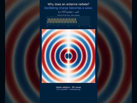
🎬 Watch it in motion
Electric Dipole | the field two opposite charges weave #Shorts