Analytically compute sloshing natural frequencies for rectangular tanks. Adjust tank width, fluid depth, and density to view 5 sloshing modes and the equivalent pendulum length in real time.
Tank Parameters
Tank width a
m
Fluid depth h
m
Fluid density ρ
kg/m³
Results
Results
—
f₁ (Hz) Mode 1
—
f₂ (Hz) Mode 2
—
Equiv. pendulum (m)
—
Pendulum period (s)
Sloshing Natural Frequencies (Modes 1–5)
Tank Cross-Section — Mode 1 Standing Wave Animation
What exactly is "sloshing" in a tank? Is it just the water sloshing back and forth when I carry a full bucket?
🎓
Basically, yes! But in engineering, we care about the precise, rhythmic waves that form inside large containers like fuel tanks or water towers when they're shaken. In practice, this isn't random splashing; it's a set of predictable natural frequencies, just like a guitar string has specific notes. Try moving the "Fluid Depth" slider above—you'll see how the sloshing frequency changes dramatically.
🙋
Wait, really? So the tank has "notes"? What controls which "note" or mode I get?
🎓
Exactly! The main controls are the tank's width and how full it is. For instance, a wide, shallow tank will have a much slower, lower-frequency slosh than a narrow, deep one. The simulator shows the first five modes (n=1,2,3,4,5). Mode 1 is the basic, whole-tank slosh. When you change the "Tank Width" parameter, you're directly changing the wavelength of these standing waves inside.
🙋
That pendulum equation in the theory box seems weird. Why compare sloshing to a pendulum?
🎓
Great observation! It's a brilliant simplification. A common case in seismic design is that the complex fluid motion in the first mode behaves as if it were a solid mass on a pendulum of a specific length. This "Equivalent Pendulum Length" lets structural engineers model sloshing forces easily without simulating the entire fluid. Adjust the fluid depth in the simulator and watch how the equivalent length changes—it's a key result for design.
Physical Model & Key Equations
The core of the analysis is finding the natural frequencies of standing surface waves in a rectangular tank. The frequency for each sloshing mode 'n' is governed by gravity, the wave number, and the fluid depth.
$f_n$: Natural frequency of mode n (Hz) $g$: Acceleration due to gravity (9.81 m/s²) $k_n$ : Wave number for mode n = $n\pi / a$ $a$: Tank width (m) $h$: Fluid depth (m)
The $\tanh(k_n h)$ function captures the effect of finite fluid depth—it transitions from shallow to deep water behavior.
For engineering design, the fundamental (n=1) sloshing mode is often modeled as a simple pendulum. This equivalent pendulum length allows the complex fluid dynamics to be represented as a simple oscillating mass in structural calculations.
$l_{eq}$: Equivalent pendulum length (m).
This length tells you how "long" the pendulum would be to swing at the same frequency as the liquid's first sloshing mode. A shorter $l_{eq}$ means a faster, more violent slosh for a given tank geometry.
Frequently Asked Questions
Increasing the tank width reduces the wave number, lowering the natural frequency. Increasing the liquid depth brings the tanh term closer to 1, increasing the frequency, but it saturates once the depth becomes sufficiently large. Caution is needed at shallow liquid depths, as the frequency drops sharply.
The equivalent pendulum length is the length used when modeling the fundamental sloshing mode as a simple pendulum. This value can be used for tank vibration damping design or for replacing it with a spring-mass model in seismic response analysis.
This tool provides theoretical values assuming small amplitude and an ideal rectangular tank. In actual design, it is necessary to consider the effects of tank elastic deformation, internal structures, and nonlinear effects. Use it as a reference and verify details through FEM or experiments.
Typically, the fundamental mode (n=1) is the most easily excited and important. However, when the excitation frequency of the tank matches a higher-order mode, or in vibration damping design, the second and third modes may also be considered. Use this tool to understand trends and select evaluation targets as needed.
Real-World Applications
Seismic Design of Storage Tanks: This is the most critical application. During an earthquake, sloshing can generate enormous forces on tank walls and roofs. Standards like API 650 use the equivalent pendulum method to calculate these "convective" forces and ensure tanks in refineries or water treatment plants don't fail.
Aerospace Propellant Management: In rockets, sloshing of liquid fuel can destabilize the vehicle's flight. Engineers must calculate sloshing frequencies to avoid matching the rocket's control system frequencies, which could lead to a destructive feedback loop. The analysis informs baffle design inside the tank.
Marine Cargo & Ballast Tanks: On ships, sloshing in partially filled cargo holds (for LNG, oil, or ballast water) creates dynamic loads that can fatigue the structure. Analyzing these modes helps determine safe filling levels and routing to avoid wave conditions that excite sloshing.
Automotive Fuel Tanks: In cars, sudden stops or turns can cause fuel slosh, which affects vehicle handling and can lead to fuel pump starvation. Baffles are designed using sloshing frequency analysis to dampen these motions and ensure consistent fuel delivery.
Common Misconceptions and Points to Note
When you start using this tool, there are several points, especially for CAE beginners, that are easy to stumble on. A major misconception is thinking that the calculation results are the actual design values. This simulator provides the theoretical solution for an ideal rectangular tank assuming "small amplitude". Actual tanks are often cylindrical, and when liquid surface motion becomes large, nonlinear phenomena can no longer be ignored. For example, even if the calculated natural frequency is 1.0 Hz, you should anticipate a variation of about 0.8 Hz to 1.2 Hz in the real machine.
Next, there's a pitfall in parameter input. The liquid depth "h" is the depth at rest, right? But when the tank is accelerating, the liquid surface tilts, changing the effective depth. Consider a car's fuel tank. During hard braking, if the liquid surges forward, the pressure on the rear wall becomes smaller than the calculated value. Conversely, during a turn, one side wall might experience a load greater than anticipated. You should treat simulation results as "one reference state"; in practice, it's essential to examine multiple cases assuming the most severe liquid surface orientations.
Finally, the assumption that you only need to look at the first mode. While the fundamental mode indeed has the most energy, higher-order modes cannot be ignored in some situations. For instance, small internal structures (like mounting struts for measurement equipment) might be located at the nodes (points of minimal motion) or antinodes (points of large motion) of the 3rd or 5th mode waves locally. Understand the purpose of visualizing up to 5 modes with this tool, and get into the habit of considering which modes affect your specific design object.
Enter tank length (m) in the input field and adjust with sl-a slider
Set fluid depth (m) in the input field and adjust with sl-h slider
Input liquid density (kg/m³) in the input field for accurate mass calculation
Simulator computes first five sloshing modes using shallow-water wave theory
Read fundamental frequency f₁ and secondary mode f₂ in Hz output fields
Review equivalent pendulum length and period for comparison to simple pendulum behavior
Worked Example
Rectangular tank carrying liquefied natural gas: length A = 8 m, fluid depth H = 2.5 m, density ρ = 420 kg/m³. First symmetric mode (n=1) frequency f₁ = 0.47 Hz calculated from f = (n·g·tanh(n·π·H/A))/(2π·A)^0.5. Second mode f₂ = 0.94 Hz. Equivalent pendulum length = 11.2 m, period = 6.7 s. When tank accelerates horizontally at 0.2 g, dominant 0.47 Hz resonance dominates sloshing response, critical for structural coupling analysis.
Practical Notes
Shallow-water approximation applies when H/A < 0.3; for deeper tanks, Boussinesq corrections improve accuracy
Sloshing frequencies drop significantly in long tanks—doubling length A reduces f₁ by ~29%, increasing damping design demands
Density affects added mass, not frequency; use ρ = 1000 kg/m³ for freshwater, 1025 for seawater, 420 for LNG
Excitation near f₁ or f₂ triggers resonant amplification; ship accelerations typically 0.05–0.15 g at these natural frequencies
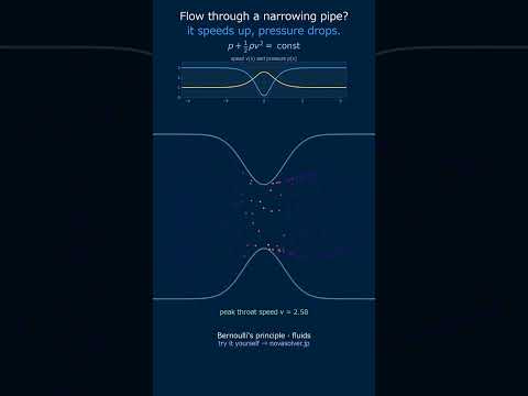
🎬 Watch it in motion
Flow speeds up in narrow spots — Bernoulli's principle #Shorts