ASME V&V 20: CFD Verification and Validation
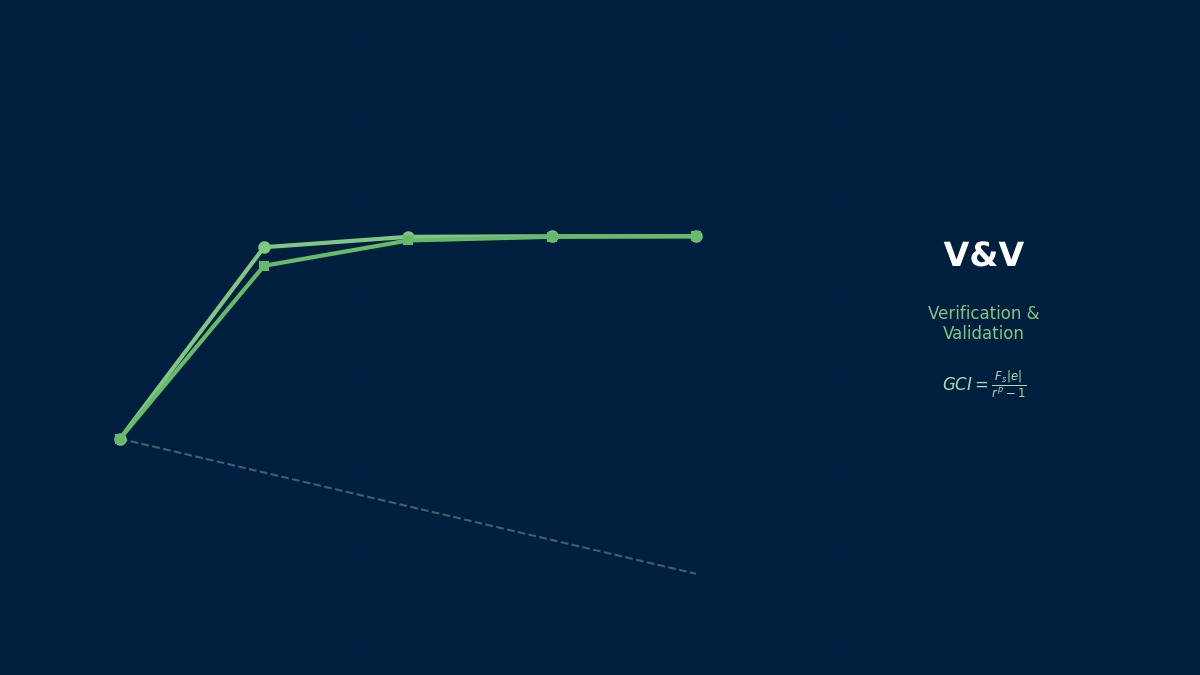
Concept: compare the difference with the uncertainty
Overview
Our CFD result came out 5% above the experiment. My manager wants to know whether the model is wrong or the experiment is just scattered.
ASME V&V 20 defines the procedure for exactly that question. The simulation–experiment difference mixes the model's own error with numerical error from finite grids, uncertainty in inputs and experimental measurement error. You estimate how large the three non-model contributions could be, combine them, and only when the difference is clearly larger can you say the model has an error. The point is not to judge from the size of the difference alone.
Decomposing the comparison error
$S$ is the simulation result, $D$ the experimental value and $E$ the comparison error. The right side is the sum of model error $\delta_{model}$, numerical error $\delta_{num}$, input-induced error $\delta_{input}$ and experimental error $\delta_D$. We want $\delta_{model}$, but the other three are not known exactly, so they are treated as uncertainties (sizes of spread).
Validation uncertainty
$u_{val}$ combines the three uncertainties by root-sum-square. The model error is estimated to lie within $E \pm k\,u_{val}$ ($k$ is a coverage factor, often 2). If that interval includes zero, the model error is buried in the uncertainty and cannot be distinguished.
Why verification and validation were separated
When CFD entered design work in the 1980s–90s, “the calculation is right” meant two different things: are we solving the equations correctly (verification), and are we solving the right equations (validation)? The first is mathematics and can be checked by refining grids; the second is physics and can only be checked against experiment. Around then, journals began refusing papers that did not demonstrate grid convergence, and that movement culminated in V&V 20 in 2009.
Worked example: Nusselt number in a heated pipe
Step 1: numerical uncertainty (three grids)
The following is an illustrative example. On three grids each halving the spacing ($r = 2$), the Nusselt number is 101.2, 102.0 and 104.8 from fine to coarse. The observed order is $p = 1.81$ and the fine-grid GCI is 0.40% (0.40). Here the GCI is treated as roughly a 95% band and halved, giving $u_{num} = 0.20$.
Step 2: input uncertainty
The Nusselt number scales roughly as Reynolds number to the 0.8 and Prandtl number to the 0.4, so the sensitivity coefficients are 0.8 and 0.4. With 1.5% uncertainty in Reynolds number (flow rate) and 2% in Prandtl number (properties), the contributions are 1.21 and 0.81, combining to $u_{input} = 1.46$.
Step 3: comparison and judgement
With $D = 96.0$ and $S = 101.2$, $E = 5.2$ (5.4% of the experiment). Two experimental uncertainties, 3% and 1%, are compared:
| Experimental uncertainty | u_D | u_val | E / u_val | Model-error interval (k=2) | Verdict |
|---|---|---|---|---|---|
| 3 % | 2.88 | 3.23 | 1.61 | −1.3 – 11.7 | Indistinguishable |
| 1 % | 0.96 | 1.76 | 2.96 | 1.7 – 8.7 | Model error present |
The same 5.4% difference, yet the conclusion flips depending on the experiment's accuracy.
Right. At 3% experimental uncertainty, 79% of the variance comes from the experiment and less than 1% from numerics — no amount of grid refinement changes the verdict. At 1%, input uncertainty takes 69% and becomes dominant. Looking at the breakdown tells you what to improve next — experiment, properties or grid. That is the most practically useful part of V&V 20.
Practical workflow
Procedure
- Choose the quantity to compare — something measurable that matters for design, such as wall heat flux or pressure drop.
- Complete code verification against known solutions, then obtain numerical uncertainty on at least three grids.
- Obtain sensitivity coefficients for each input; tighten those with both high sensitivity and high uncertainty first.
- Get the experimental uncertainty estimate — including repeatability, not just instrument accuracy.
- Compare $E$ with $u_{val}$ and report the breakdown.
Cautions
- Asymptotic range: if the observed order is far from the theoretical one or differences change sign, don't trust the GCI as is.
- Correlated inputs: inputs that are not independent, such as related properties, cannot simply be combined by root-sum-square.
- Don't judge from one point: compare at several conditions to see trends in model error.
Tuning is not validation
Adjusting turbulence-model constants or wall roughness until the simulation matches the experiment is common practice — but from the V&V 20 standpoint it is not validation. The error looks like zero at the tuned point, yet checking against the data used for tuning proves nothing. Only comparison with data at conditions not used for tuning reveals predictive power. Reports should state separately which data were used for tuning and which for validation.
Common mistakes
Mistakes and fixes
| Mistake | Effect | Fix |
|---|---|---|
| Judging by the difference alone | Changing the model wrongly | Compare E with u_val |
| Concluding from one grid | Numerical error unknown | GCI on three or more grids |
| Treating data as truth | u_D ignored, uncertainty underestimated | Obtain experimental uncertainty |
| Validating with tuning data | Predictive power overstated | Compare at other conditions |
| No breakdown reported | Next improvement unclear | Show variance shares |
I'd like to try GCI and uncertainty combination myself.
Try the Richardson extrapolation tool and mesh convergence tool for convergence order and GCI, and the uncertainty propagation tool for how input uncertainty propagates. See Roache's GCI, solution verification and validation metrics for details, and ASME V&V 10 for the structural-mechanics counterpart.