What is multiphysics uncertainty quantification?

Determining how much scatter in inputs — material values, boundary conditions, loads — produces in the results of a coupled analysis. Because physics interact, one input's scatter can be amplified, making it more important than in single-physics analysis.

How much does coupling widen the scatter?

For the example copper wire (1 mm², 20 A), the same input scatter gives a 5–95% temperature range of 104–157 °C without temperature-dependent resistance, but 139–292 °C with coupling. The positive feedback — higher temperature, higher resistance, more heat — amplifies the scatter.

Which methods are used?

Monte Carlo, repeating the calculation with sampled inputs, is the baseline. Linear estimates from sensitivities are fast but fail under strong nonlinearity: in the example the linearised standard deviation was 39 K, while the Monte Carlo distribution had a long high-temperature tail and a far higher 95th percentile. For expensive models, response surfaces or reduced-order models are used.

Multiphysics Uncertainty Quantification

Category: Coupled Analysis | Revised 2026-09-30

CAE visualization for uncertainty multiphysics theory - technical simulation diagram

Uncertainty Quantification for Multiphysics

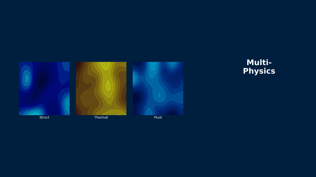
Concept: input scatter propagates to results

Overview

🙋

A coupled analysis gives me a single number, but material values and heat transfer coefficients are quite uncertain. How far can I trust the result?

🎓

Uncertainty quantification answers that in numbers: vary each input within its range and find how much the result scatters. What matters especially in coupled analysis is that interactions between physics can amplify scatter. A current-heated wire gains resistance as it warms and heats further, so a slightly lower heat transfer coefficient can raise temperature a lot. The single-physics instinct that ±15% in, ±15% out will mislead you.

Main methods

$$ \sigma_Y^2 \approx \sum_i \left(\frac{\partial Y}{\partial X_i}\right)^2 \sigma_{X_i}^2 $$

$$ \hat{\mu}_Y = \frac{1}{N}\sum_{n=1}^{N} Y\big(\mathbf{X}^{(n)}\big), \qquad \text{standard error} \approx \frac{\sigma_Y}{\sqrt{N}} $$

The first is linearisation, estimating standard deviation from sensitivities (partial derivatives); it needs only one more run than the number of inputs but errs under strong nonlinearity. The second is Monte Carlo, running $N$ sampled cases; it handles any nonlinearity but the error of the mean falls only as $1/\sqrt{N}$, so many runs are needed.

The coupled problem used here

$$ T = T_a + \frac{I^2 \rho_{20}\,[1 + \alpha(T-20)]}{A\,h\,\pi d} $$

A bare 1 mm² copper wire carries 20 A and loses heat from its surface with coefficient $h$. Temperature-dependent resistance (coefficient $\alpha$) couples temperature and heating. See resistive heating analysis for details.

Coffee Break Trivia

A method born in weapons research

The Monte Carlo method emerged in the 1940s from neutron-diffusion research at Los Alamos. The mathematician Ulam reportedly realised it was faster to estimate the odds of winning a game of solitaire by dealing it many times than by calculation. Von Neumann and colleagues named it after the Monaco district famous for its casino. What was once a few hundred trials on early computers is now hundreds of thousands in seconds on a laptop — though when one coupled run takes hours, the number of runs is still a serious constraint.

Worked example: scatter of wire temperature

Input scatter

Input	Mean	Standard deviation
Heat transfer coefficient h	20 W/(m²·K)	3 (15%)
Current I	20 A	0.2 (1%)
Resistivity ρ₂₀	1.72×10⁻⁸ Ω·m	1%
Ambient Ta	25 ℃	2 K

Monte Carlo results (200,000 samples)

Model	Nominal	Mean	5th pct	Median	95th pct
Uncoupled (constant R)	123.9 ℃	126.4 ℃	103.7 ℃	124.0 ℃	156.9 ℃
Coupled	184.9 ℃	197.5 ℃	138.6 ℃	185.1 ℃	291.9 ℃

🙋

With coupling, the 95th percentile is over 100 K above nominal.

🎓

Right. Uncoupled, the 95th percentile is 33 K above nominal; coupled, it is 107 K above. When the heat transfer coefficient swings low, temperature rises, resistance grows and heating increases further, so the distribution stretches toward high temperature, and even the mean shifts about 13 K above nominal. With a 150 °C insulation limit, the probability of exceeding it is about 9% uncoupled and about 87% coupled — a clear warning against judging from one nominal value.

Which inputs matter

Variance shares from sensitivities at the nominal point: heat transfer coefficient 97%, current 2%, ambient 1%, resistivity nearly 0%. To reduce scatter, pinning down the heat transfer coefficient (cooling conditions) experimentally beats remeasuring material values. But the linearised standard deviation of 39 K fails to capture the Monte Carlo spread; it is useful for ranking inputs, while probability estimates need Monte Carlo.

Practical workflow

Procedure

Set range and distribution for each input; without data, use literature or experience and record the basis.
Screen influential inputs by sensitivity analysis; a few usually dominate.
Run Monte Carlo on the key inputs; for expensive models, substitute response surfaces or reduced-order models.
Judge by exceedance probability and upper percentiles, not just mean and standard deviation.

Coffee Break Trivia

“A safety margin from the standard deviation fell short”

Adding twice the standard deviation to the nominal value as a conservative figure is common practice. That works for near-symmetric normal distributions, but positive feedback in coupled problems stretches the distribution toward high values. For the example wire, nominal 185 °C plus twice the linearised 39 K gives about 264 °C, whereas the Monte Carlo 95th percentile is 292 °C and the 99th 397 °C. Mean and standard deviation don't reveal the tail; compute the percentile you actually decide on.

Common mistakes

Mistakes and fixes

Mistake	Effect	Fix
Judging on one nominal value	Exceedance probability missed	Obtain the distribution
Linearisation only	Tail underestimated	Confirm with Monte Carlo
Varying every input	Too many runs	Screen by sensitivity
UQ with coupling removed	Scatter underestimated	Use the coupled model
No basis for input ranges	Can't justify results	Record sources and assumptions

🙋

I'd like to try Monte Carlo and uncertainty propagation myself.

🎓

Try the Monte Carlo statistics tool for Monte Carlo and the uncertainty propagation tool for linear propagation. Using UQ in comparisons with experiment is covered in ASME V&V 20, judging coupling strength in strong versus weak coupling, and ways to make runs cheaper in reduced-order models.

Rate this article

Thank you for your feedback!

Helpful

More details

Report error