Theoretical, Numerical Analysis, and Practical Guide to Dipole Antennas
Theoretical, Numerical Analysis, and Theoretical, Numerical Analysis, and Theoretical, Numerical Analysis, and Practical Guide in Practice in Practice: Theoretical Foundations
Overview — What is a Dipole Antenna
Dipole antennas appear at the beginning of antenna textbooks, but are they actually used in practice?
They are used extensively. The rod-shaped antennas on Wi-Fi routers are exactly dipoles—well, more precisely monopoles using a ground plane, but the principle is the same. Half-wave dipoles are also standard for FM broadcasting and amateur radio antennas. Furthermore, they serve as the reference (0dBd = 2.15dBi) for measuring the gain of all other antennas. They are like the "meter prototype" of antenna engineering.
I see, so it's a fundamental antenna that serves as a benchmark. What about its structure?
Two conductor rods (elements) are aligned in a straight line, and a high-frequency signal is fed from the center. One with a total length of half the wavelength ($\lambda/2$) is called a half-wave dipole. For example, for 2.4GHz Wi-Fi, the wavelength is 125mm, so you have two conductors each about 31mm long. It's a very simple structure, but whether you can properly explain why the input impedance becomes $73 + j42.5\,\Omega$ serves as a litmus test for your understanding of electromagnetism.
Radiation from an Infinitesimal Dipole
Starting with a half-wave dipole seems difficult. Can we begin with a simpler model?
Good idea. Let's start with an infinitesimal dipole (Hertzian dipole). When a uniform current $I_0$ flows through a conductor that is sufficiently short compared to the wavelength ($l \ll \lambda$), the far-field electric field is:
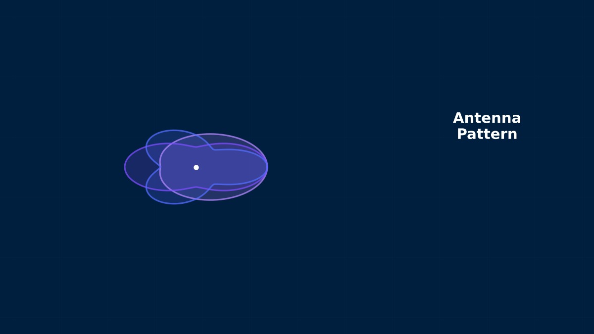
Here, $\eta_0 = 120\pi\,\Omega$ is the impedance of free space, and $k = 2\pi/\lambda$ is the wave number. The important part is the $\sin\theta$ term, which is maximum at $\theta = 90°$ (direction perpendicular to the antenna) and zero at $\theta = 0°, 180°$ (along the antenna axis). In other words, it's a doughnut-shaped radiation pattern.
What about the radiation resistance?
Integrate the Poynting vector from the far field over the entire solid angle to find the radiated power $P_{rad}$, and derive the radiation resistance from $P_{rad} = \frac{1}{2}R_{rad}|I_0|^2$:
For example, if $l = \lambda/10$, then $R_{rad} \approx 7.9\,\Omega$. The shorter the antenna relative to the wavelength, the smaller the radiation resistance, leading to poorer radiation efficiency. This is why "electrically short antennas have poor efficiency." This is also the challenge in designing antennas for mobile phones.
Current Distribution and Radiation Pattern of a Half-Wave Dipole
The infinitesimal dipole seems too idealized. How does it change for an actual half-wave dipole?
Good observation. In a half-wave dipole (total length $L = \lambda/2$), the current distribution is not uniform but sinusoidal:
Maximum $I_0$ at the center (feed point), zero at both ends. Calculating the far field from this current distribution yields:
Compared to the $\sin\theta$ of the infinitesimal dipole, $\cos(\frac{\pi}{2}\cos\theta)/\sin\theta$ results in a slightly "tighter" pattern. The direction of maximum radiation ($\theta = 90°$) is the same, but the nulls along the axis are deeper. This difference appears as a difference in directivity.
It makes intuitive sense that the current is zero at the ends. It's an open end, so there's no path for current to flow, right?
Exactly. It's the same boundary condition as the open end of a transmission line. The current is zero, but the voltage (electric field) is maximum. The fact that this voltage/current distribution forms a standing wave is the essence of the dipole, and the view that "an antenna is an opened transmission line" holds true.
Derivation of Radiation Resistance 73Ω and Input Impedance
73Ω is a rather odd number. Why does it become that?
Calculate the Poynting vector $\mathbf{S} = \frac{1}{2\eta_0}|E_\theta|^2 \hat{r}$ from the far field $E_\theta$ and integrate over the entire sphere to obtain the radiated power:
This integral cannot be solved analytically in closed form; numerical integration yields approximately 1.219. From $P_{rad} = \frac{1}{2}R_{rad}|I_0|^2$:
This calculation result is what's written as "approximately 73Ω" in electromagnetism textbooks. It's slightly mismatched with 50Ω coaxial cable but quite close to 75Ω cable. In fact, the 75Ω impedance for television has a history of being determined to match the radiation resistance of the half-wave dipole.
The input impedance is $73 + j42.5\,\Omega$; where does the imaginary part come from?
The antenna's near field has a reactive component that stores energy. Exactly at half-wavelength ($L = \lambda/2$), the stored electric field energy slightly exceeds the magnetic field energy, resulting in an inductive (positive reactance $j42.5\,\Omega$) component.
In practice, to cancel this reactance and make it purely resistive, the antenna length is shortened to about $0.47\lambda$~$0.48\lambda$. Then the reactance becomes zero and $Z_{in} \approx 73\,\Omega$ (pure resistance). This "resonant length" varies slightly depending on wire diameter and surrounding environment, so it's common to fine-tune it with simulation.
Physical Meaning of Directivity 1.64 (2.15dBi)
I often see 2.15dBi in antenna catalogs, but what does it specifically represent?
Directivity $D$ is the ratio of "radiation intensity in the maximum radiation direction" to "radiation intensity if radiated equally in all directions":
For a half-wave dipole, $D = 1.643$. Expressed in dB:
This means "approximately 64% stronger in the strongest direction compared to an isotropic antenna." Even with the exact same input power, because it's concentrated in the equatorial direction of the doughnut, it becomes stronger only in that direction. Yagi antennas (TV antennas) have gains like 10dBi or 12dBi because they further narrow the beam based on the dipole.
The "i" in dBi stands for isotropic, right? I also see the notation dBd sometimes.
dBd is gain relative to a half-wave dipole as reference. That is, $0\,\mathrm{dBd} = 2.15\,\mathrm{dBi}$. dBd is often used in the amateur radio world, but dBi is standard in academic papers and CAE. Just remember the conversion: $G_{\mathrm{dBi}} = G_{\mathrm{dBd}} + 2.15$.
Hertz's Experiment (1888) — The First "Antenna" Was a Dipole
In 1888, Heinrich Hertz succeeded for the first time in transmitting and receiving electromagnetic waves using two metal rods (exactly a dipole). It was a simple experiment: exciting high-frequency oscillation with a spark discharge and observing the induced spark in a receiving dipole several meters away, but it was the historic moment that first demonstrated Maxwell's theoretical prediction. The wavelength was about 66cm, equivalent to what we now call the 450MHz band. Hertz denied the practical value of this discovery, but about 10 years later, Marconi applied it to wireless communication and changed the world.
Numerical Solution Method and Implementation
Details of Numerical Methods
Specifically, what algorithm is used to solve for a dipole antenna?
Now I understand what my senior meant when he said, "At least do it properly for the dipole antenna."
Formulation of Discretization
Approximate the unknown quantity using shape functions $N_i$:
Expressing this mathematically gives:
Discrete Form of the Governing Equations
Expressing this mathematically gives:
Hmm, just equations don't really click... What do they represent?
Discretizing the governing equations of the continuum yields the following system of algebraic equations:
Here, $[K]$ is the global stiffness matrix (or equivalent system matrix), $\{u\}$ is the vector of unknown nodal variables, and $\{F\}$ is the external force vector.
Ah, I see! So that's the mechanism behind "discretizing the governing equations of the continuum."
Element Technology
I've heard of "element technology," but I might not fully understand it...
| Element Type | Order | Number of Nodes (3D) | Accuracy | Computational Cost |
|---|---|---|---|---|
| Tetrahedron Linear | Linear | 4 | Low (Shear Locking) | Low |
| Tetrahedron Quadratic | Quadratic | 10 | High | Medium |
| Hexahedron Linear | Linear | 8 | Medium | Medium |
| Hexahedron Quadratic | Quadratic | 20 | Very High | High |
| Prism | Linear/Quadratic | 6/15 | Medium–High | Medium |
Integration Scheme
What exactly is an integration scheme?
- Full Integration: Integrates all terms accurately. Tends to overestimate stiffness (Locking).
- Reduced Integration: Reduces the number of integration points. Improves computational efficiency but risks hourglass mode generation.
- Selective Reduced Integration (B-bar Method): Separates and integrates volumetric and deviatoric terms. Avoids locking.
After hearing this, I finally understand why element type is so important!
Convergence and Stability
If it stops converging, what should I check first?
- h-refinement: Refine the mesh (reduce element size h) to improve accuracy.
- p-refinement: Increase the polynomial order of elements to improve accuracy.
- hp-refinement: Simultaneously optimize h and p.
Related Topics
Experience the theory firsthand with the interactive simulator for this field
All Simulators