Natural Convection CFD Analysis
Theory and Physics
Fundamentals of Natural Convection
Professor, natural convection is when flow occurs without an external power source, right? What is the driving force?
It's buoyancy. The density of the fluid changes with temperature, and in a gravitational field, this density difference creates a pressure imbalance, which generates flow. Fluid in the high-temperature region becomes less dense and rises, while fluid in the low-temperature region descends. This circulation is natural convection.
What is the indicator that represents the strength of natural convection?
The Rayleigh number $Ra$ is the fundamental indicator.
Here, $g$ is gravitational acceleration, $\beta$ is the volumetric expansion coefficient, $\Delta T$ is the temperature difference, $L$ is the characteristic length, $\nu$ is the kinematic viscosity, $\alpha$ is the thermal diffusivity. It is the product of the Grashof number $Gr$ and the Prandtl number $Pr$.
The flow regime is divided by $Ra$. For a vertical flat plate, $Ra < 10^9$ is laminar, $Ra > 10^9$ is turbulent. In an enclosed cavity, transition to unsteady flow occurs around $Ra > 10^8$.
Boussinesq Approximation
What exactly is the assumption of the Boussinesq approximation?
It's an approximation applicable when density fluctuations are sufficiently small compared to a reference density ($\beta \Delta T \ll 1$). It considers density variation only in the buoyancy term of the momentum equation, while treating density as constant in the continuity equation.
$$ \rho \approx \rho_0 [1 - \beta(T - T_0)] $$
For air, a safe application range is typically $\Delta T < 30$°C. For water, since the volumetric expansion coefficient has temperature dependence, a polynomial density model should be used for wide temperature ranges.
Coffee Break Casual Talk
The World of "Turbulent Natural Convection" Beyond Rayleigh Number 10⁹
The flow regime in natural convection changes dramatically with the Rayleigh number (Ra = Gr × Pr). For Ra < 10⁸, stable laminar convection cells form, and the correlation for the Nusselt number is relatively simple. However, when Ra > 10⁹, turbulence begins, and the prediction accuracy of the Nu number plummets. This scale corresponds to "building exterior walls heated by sunlight" or "oil cooling for large transformers"—conditions commonly encountered in practice. In turbulent natural convection, plume-like structures near walls randomly generate and vanish, often causing steady-state analyses to fail to converge. In such cases, switching to a strategy of taking time averages from unsteady calculations is advisable.
Physical Meaning of Each Term
- Time Term $\partial(\rho\phi)/\partial t$: Imagine the moment you turn on a faucet. At first, water comes out in an unstable, splashing manner, but after a while, it becomes a steady flow, right? This "period of change" is described by the time term. The pulsation of blood flow from a heartbeat, or flow fluctuations each time an engine valve opens and closes—all are unsteady phenomena. So what is steady-state analysis? It looks only at "after sufficient time has passed and the flow has settled down"—meaning setting this term to zero. Since computational cost drops significantly, trying a steady-state solution first is a basic CFD strategy.
- Convection Term $\nabla \cdot (\rho \mathbf{u} \phi)$: What happens if you drop a leaf into a river? It gets carried downstream by the flow, right? This is "convection"—the effect where fluid motion transports things. Warm air from a heater reaching the far corner of a room is also because the air, as a "carrier," transports heat via convection. Here's the interesting part—this term contains "velocity × velocity," making it nonlinear. That is, as flow speed increases, this term rapidly strengthens, making control difficult. This is the root cause of turbulence. A common misconception: "Convection and conduction are similar things" → They are completely different! Convection is carried by flow, conduction is transmitted by molecules. There's an order-of-magnitude difference in efficiency.
- Diffusion Term $\nabla \cdot (\Gamma \nabla \phi)$: Have you ever put milk in coffee and left it? Even without stirring, after a while, it naturally mixes, right? That's molecular diffusion. Now, a question—honey and water, which flows more easily? Obviously water, right? Honey has high viscosity ($\mu$), so it flows poorly. Higher viscosity strengthens the diffusion term, making the fluid move in a "thick" manner. In low Reynolds number flows (slow, viscous), diffusion dominates. Conversely, in high Re number flows, convection overwhelms, and diffusion plays a supporting role.
- Pressure Term $-\nabla p$: When you push the plunger of a syringe, liquid shoots out forcefully from the needle tip, right? Why? The piston side is high pressure, the needle tip is low pressure—this pressure difference provides the force that pushes the fluid. Dam discharge works on the same principle. On a weather map, where isobars are tightly packed? That's right, strong winds blow. "Flow is generated where there is a pressure difference"—this is the physical meaning of the pressure term in the Navier-Stokes equations. A point of confusion here: "Pressure" in CFD is often gauge pressure, not absolute pressure. When you switch to a compressible analysis and suddenly get strange results, it might be due to mixing up absolute/gauge pressure.
- Source Term $S_\phi$: Heated air rises—why? Because it becomes lighter (less dense) than its surroundings, so it's pushed up by buoyancy. This buoyancy is added to the equation as a source term. Other examples: chemical reaction heat from a gas stove flame, Lorentz force acting on molten metal in a factory's electromagnetic pump... These are all actions that "inject energy or force into the fluid from the outside," expressed by source terms. What happens if you forget a source term? In a natural convection analysis, forgetting buoyancy means the fluid doesn't move at all—a physically impossible result like turning on a heater in a winter room but the warm air doesn't rise.
Assumptions and Applicability Limits
- Continuum Assumption: Valid for Knudsen number Kn < 0.01 (mean free path ≪ characteristic length)
- Newtonian Fluid Assumption: Shear stress and strain rate have a linear relationship (non-Newtonian fluids require viscosity models)
- Incompressibility Assumption (for Ma < 0.3): Treat density as constant. For Mach numbers above 0.3, compressibility effects must be considered
- Boussinesq Approximation (Natural Convection): Consider density variation only in the buoyancy term, using constant density in other terms
- Non-applicable Cases: Rarefied gases (Kn > 0.1), supersonic/hypersonic flow (shock capturing required), free surface flow (VOF/Level Set, etc., required)
Dimensional Analysis and Unit Systems
Variable SI Unit Notes / Conversion Memo
Velocity $u$ m/s When converting from volumetric flow rate for inlet conditions, pay attention to cross-sectional area units
Pressure $p$ Pa Distinguish between gauge and absolute pressure. Use absolute pressure for compressible analysis
Density $\rho$ kg/m³ Air: ~1.225 kg/m³ @20°C, Water: ~998 kg/m³ @20°C
Viscosity $\mu$ Pa·s Be careful not to confuse with kinematic viscosity $\nu = \mu/\rho$ [m²/s]
Reynolds Number $Re$ Dimensionless $Re = \rho u L / \mu$. Indicator for laminar/turbulent transition
CFL Number Dimensionless $CFL = u \Delta t / \Delta x$. Directly related to time step stability
What exactly is the assumption of the Boussinesq approximation?
It's an approximation applicable when density fluctuations are sufficiently small compared to a reference density ($\beta \Delta T \ll 1$). It considers density variation only in the buoyancy term of the momentum equation, while treating density as constant in the continuity equation.
For air, a safe application range is typically $\Delta T < 30$°C. For water, since the volumetric expansion coefficient has temperature dependence, a polynomial density model should be used for wide temperature ranges.
The World of "Turbulent Natural Convection" Beyond Rayleigh Number 10⁹
The flow regime in natural convection changes dramatically with the Rayleigh number (Ra = Gr × Pr). For Ra < 10⁸, stable laminar convection cells form, and the correlation for the Nusselt number is relatively simple. However, when Ra > 10⁹, turbulence begins, and the prediction accuracy of the Nu number plummets. This scale corresponds to "building exterior walls heated by sunlight" or "oil cooling for large transformers"—conditions commonly encountered in practice. In turbulent natural convection, plume-like structures near walls randomly generate and vanish, often causing steady-state analyses to fail to converge. In such cases, switching to a strategy of taking time averages from unsteady calculations is advisable.
Physical Meaning of Each Term
- Time Term $\partial(\rho\phi)/\partial t$: Imagine the moment you turn on a faucet. At first, water comes out in an unstable, splashing manner, but after a while, it becomes a steady flow, right? This "period of change" is described by the time term. The pulsation of blood flow from a heartbeat, or flow fluctuations each time an engine valve opens and closes—all are unsteady phenomena. So what is steady-state analysis? It looks only at "after sufficient time has passed and the flow has settled down"—meaning setting this term to zero. Since computational cost drops significantly, trying a steady-state solution first is a basic CFD strategy.
- Convection Term $\nabla \cdot (\rho \mathbf{u} \phi)$: What happens if you drop a leaf into a river? It gets carried downstream by the flow, right? This is "convection"—the effect where fluid motion transports things. Warm air from a heater reaching the far corner of a room is also because the air, as a "carrier," transports heat via convection. Here's the interesting part—this term contains "velocity × velocity," making it nonlinear. That is, as flow speed increases, this term rapidly strengthens, making control difficult. This is the root cause of turbulence. A common misconception: "Convection and conduction are similar things" → They are completely different! Convection is carried by flow, conduction is transmitted by molecules. There's an order-of-magnitude difference in efficiency.
- Diffusion Term $\nabla \cdot (\Gamma \nabla \phi)$: Have you ever put milk in coffee and left it? Even without stirring, after a while, it naturally mixes, right? That's molecular diffusion. Now, a question—honey and water, which flows more easily? Obviously water, right? Honey has high viscosity ($\mu$), so it flows poorly. Higher viscosity strengthens the diffusion term, making the fluid move in a "thick" manner. In low Reynolds number flows (slow, viscous), diffusion dominates. Conversely, in high Re number flows, convection overwhelms, and diffusion plays a supporting role.
- Pressure Term $-\nabla p$: When you push the plunger of a syringe, liquid shoots out forcefully from the needle tip, right? Why? The piston side is high pressure, the needle tip is low pressure—this pressure difference provides the force that pushes the fluid. Dam discharge works on the same principle. On a weather map, where isobars are tightly packed? That's right, strong winds blow. "Flow is generated where there is a pressure difference"—this is the physical meaning of the pressure term in the Navier-Stokes equations. A point of confusion here: "Pressure" in CFD is often gauge pressure, not absolute pressure. When you switch to a compressible analysis and suddenly get strange results, it might be due to mixing up absolute/gauge pressure.
- Source Term $S_\phi$: Heated air rises—why? Because it becomes lighter (less dense) than its surroundings, so it's pushed up by buoyancy. This buoyancy is added to the equation as a source term. Other examples: chemical reaction heat from a gas stove flame, Lorentz force acting on molten metal in a factory's electromagnetic pump... These are all actions that "inject energy or force into the fluid from the outside," expressed by source terms. What happens if you forget a source term? In a natural convection analysis, forgetting buoyancy means the fluid doesn't move at all—a physically impossible result like turning on a heater in a winter room but the warm air doesn't rise.
Assumptions and Applicability Limits
- Continuum Assumption: Valid for Knudsen number Kn < 0.01 (mean free path ≪ characteristic length)
- Newtonian Fluid Assumption: Shear stress and strain rate have a linear relationship (non-Newtonian fluids require viscosity models)
- Incompressibility Assumption (for Ma < 0.3): Treat density as constant. For Mach numbers above 0.3, compressibility effects must be considered
- Boussinesq Approximation (Natural Convection): Consider density variation only in the buoyancy term, using constant density in other terms
- Non-applicable Cases: Rarefied gases (Kn > 0.1), supersonic/hypersonic flow (shock capturing required), free surface flow (VOF/Level Set, etc., required)
Dimensional Analysis and Unit Systems
| Variable | SI Unit | Notes / Conversion Memo |
|---|---|---|
| Velocity $u$ | m/s | When converting from volumetric flow rate for inlet conditions, pay attention to cross-sectional area units |
| Pressure $p$ | Pa | Distinguish between gauge and absolute pressure. Use absolute pressure for compressible analysis |
| Density $\rho$ | kg/m³ | Air: ~1.225 kg/m³ @20°C, Water: ~998 kg/m³ @20°C |
| Viscosity $\mu$ | Pa·s | Be careful not to confuse with kinematic viscosity $\nu = \mu/\rho$ [m²/s] |
| Reynolds Number $Re$ | Dimensionless | $Re = \rho u L / \mu$. Indicator for laminar/turbulent transition |
| CFL Number | Dimensionless | $CFL = u \Delta t / \Delta x$. Directly related to time step stability |
Numerical Methods and Implementation
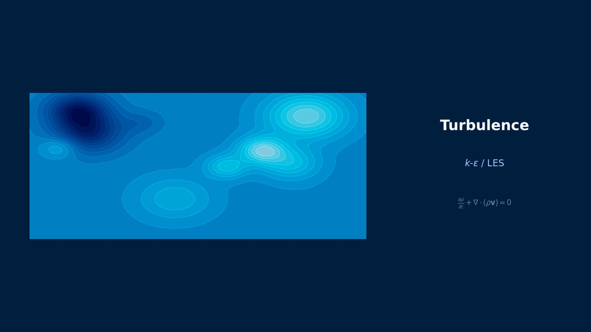
Turbulence Modeling for Natural Convection
I've heard that selecting a turbulence model for natural convection is difficult.
Compared to forced convection, natural convection has lower turbulence intensity and a wider transition region. The standard k-ε model tends to produce excessive turbulent diffusion and overestimate the Nu number. The recommended order is as follows.
| Rayleigh Number Range | Recommended Model | Notes |
|---|---|---|
| $Ra < 10^9$ | Laminar (Laminar Model) | Turbulence model not required |
| $10^9 < Ra < 10^{12}$ | SST k-ω + Low-Re Wall Treatment | Wall first layer $y^+ < 1$ mandatory |
| $Ra > 10^{12}$ | SST k-ω or Realizable k-ε | Enhanced Wall Treatment |
Can't wall functions be used for natural convection?
They should generally be avoided. The velocity and temperature profiles near walls in natural convection differ from the logarithmic law of forced convection, making standard wall functions less applicable. The Low-Re approach with $y^+ \approx 1$ is recommended. Fluent's Enhanced Wall Treatment automatically switches based on $y^+$, but for natural convection, ensuring $y^+ < 1$ is the best practice.
Mesh Design
What should I be careful about when designing a mesh for natural convection?
Estimate the thickness of the thermal and velocity boundary layers and place a sufficient number of cells within each. The boundary layer thickness for natural convection can be approximated by
For example, for a vertical flat plate with $L = 0.1$m and $Ra = 10^9$, $\delta_T \approx 0.6$mm. At least 10–15 cell layers need to be placed within this thin boundary layer.
Is it okay to make the region outside the boundary layer coarse?
The core region can be relatively coarse. However, abrupt cell size changes should be avoided; a guideline is to keep the volume ratio of adjacent cells below 1.2. STAR-CCM+'s Prism Layer Mesher or Fluent's Inflation Layer can automatically refine the region near walls.
Boussinesq Approximation in Natural Convection CFD—When It Works and When It Breaks Down
The standard "Boussinesq approximation" in natural convection analysis is a technique that linearly approximates density variation only in the buoyancy term (ρ ≈ ρ₀(1-βΔT)) and treats density as constant in other terms. It stabilizes calculations and makes convergence easier, but errors become non-negligible when the temperature difference ΔT is large. As a rule of thumb, the application limit is "βΔT < 0.1 (approximately up to 10–20°C difference)." For systems with temperature differences of several hundred degrees, such as furnace combustion or solar thermal collectors, a "non-Boussinesq (variable density)" model that treats density as a full function of temperature is essential. This requires either considering low-Mach-number compressibility in a pressure-based Navier-Stokes solver or directly incorporating a density-dependent equation of state.
Upwind Scheme
First-order Upwind: Large numerical diffusion but stable. Second-order Upwind: Improved accuracy but risk of oscillations. Essential for high Reynolds number flows.
Central Differencing
Second-order accurate, but numerical oscillations occur for Pe > 2. Suitable for low Reynolds number diffusion-dominated flows.
TVD Schemes (MUSCL, QUICK, etc.)
Maintain high accuracy while suppressing numerical oscillations via limiter functions. Effective for capturing shocks or steep gradients.
Finite Volume Method vs Finite Element Method
FVM: Naturally satisfies conservation laws. Mainstream in CFD. FEM: Advantageous for complex geometries and multiphysics. Mesh-free methods like SPH are also developing.
CFL Condition (Courant Number)
Explicit method: CFL ≤ 1 is the stability condition. Implicit method: Stable even for CFL > 1, but affects accuracy and iteration count. LES: CFL ≈ 1 recommended. Physical meaning: Information should not travel more than one cell per time step.
Residual Monitoring
Convergence is typically judged when residuals for continuity, momentum, and energy equations drop by 3–4 orders of magnitude. The mass conservation residual is particularly important.
Relaxation Factors
Typical initial values: Pressure: 0.2–0.3, Velocity: 0.5–0.7. Reduce factors if divergence occurs. Increase after convergence to accelerate.
Internal Iterations for Unsteady Calculations
Iterate within each time step until a steady solution converges. Internal iteration count: 5–20 iterations is a guideline. If residuals fluctuate between time steps, review the time step size.
Analogy for the SIMPLE Method
The SIMPLE method is an "alternating adjustment" technique. First, velocity is tentatively determined (predictor step), then pressure is corrected so that mass conservation is satisfied with that velocity (corrector step), and then velocity is revised using the corrected pressure—this back-and-forth is repeated to approach the correct solution. It resembles two people leveling a shelf: one adjusts the height, the other balances it, and they repeat this alternately.
Analogy for the Upwind Scheme
The upwind scheme is a method that "stands in the river flow and prioritizes information from upstream." A person standing in a river cannot tell where the water comes from by looking downstream—it reflects the physics that upstream information determines downstream. Although it's first-order accurate, it is highly stable because it correctly captures flow direction.
Practical Guide
Enclosed Cavity Benchmark
Are there any benchmarks available for validating natural convection CFD?
The most famous is the differentially heated rectangular cavity problem by de Vahl Davis (1983). The left wall is hot, the right wall is cold, the top and bottom walls are adiabatic, and reference solutions for Nu number and flow field are provided for $Ra = 10^3$ to $10^6$. For CFD code validation, it is standard to confirm that the wall-averaged Nu number matches de Vahl Davis's values within 1%.
What are the specific values?
| $Ra$ | Average $Nu$ (de Vahl Davis) |
|---|---|
| $10^3$ | 1.118 |
| $10^4$ | 2.243 |
| $10^5$ | 4.519 |
| $10^6$ | 8.800 |
If CFD results deviate from these by more than 2%, there is likely a problem with the settings or mesh.
Natural Air Cooling Design for Electronic Devices
What kind of CFD design is done for fanless natural air cooling?
For natural convection CFD inside an enclosed enclosure, the procedure is: (1) Set the heat generation of each component as a volumetric source, (2) Set natural convection + radiation boundary conditions on the outer surface of the enclosure walls, (3) Solve for the air inside the enclosure as the fluid. In many cases, radiation contributes 30–50% of the total heat dissipation, so combining a Surface-to-Surface radiation model (Fluent's S2S, STAR-CCM+'s Surface-to-Surface Radiation) is essential.
Modeling the heat conduction of a circuit board is tough, right?
A PCB (printed circuit board) has a laminated structure of copper layers and glass epoxy layers, with thermal conductivity differing by more than 10 times between the in-plane and thickness directions. Tools specialized for electronic thermal design like Ansys Icepak have automatic anisotropic modeling functions for PCBs. With general-purpose CFD solvers, you need to manually set orthotropic thermal conductivity.
What about enclosures with ventilation holes?
Related Topics
なった
詳しく
報告