Rotational Unbalance Response
Theory and Physics
What is Rotational Unbalance?
Professor, what is rotational unbalance?
It is the centrifugal force generated when the center of mass of a rotating body is offset from the axis of rotation (eccentricity $e$). This centrifugal force excites the structure at the same frequency as the rotational speed.
It's proportional to the square of the rotational speed! The force gets larger at higher speeds.
That's why balancing (reducing imbalance) is crucial for high-speed rotating machinery. The balance quality grade (G grade) is specified in ISO 1940.
Response Analysis
The imbalance force is a synchronous excitation (1st order: $\omega$, 2nd order: $2\omega$, ...). In FEM frequency response analysis:
1. Define the imbalance force $F = me\omega^2$ as a function of rotational speed
2. Calculate the response (displacement amplitude, vibration velocity) at each rotational speed
3. Judge if the response is within allowable limits (ISO 10816, etc.)
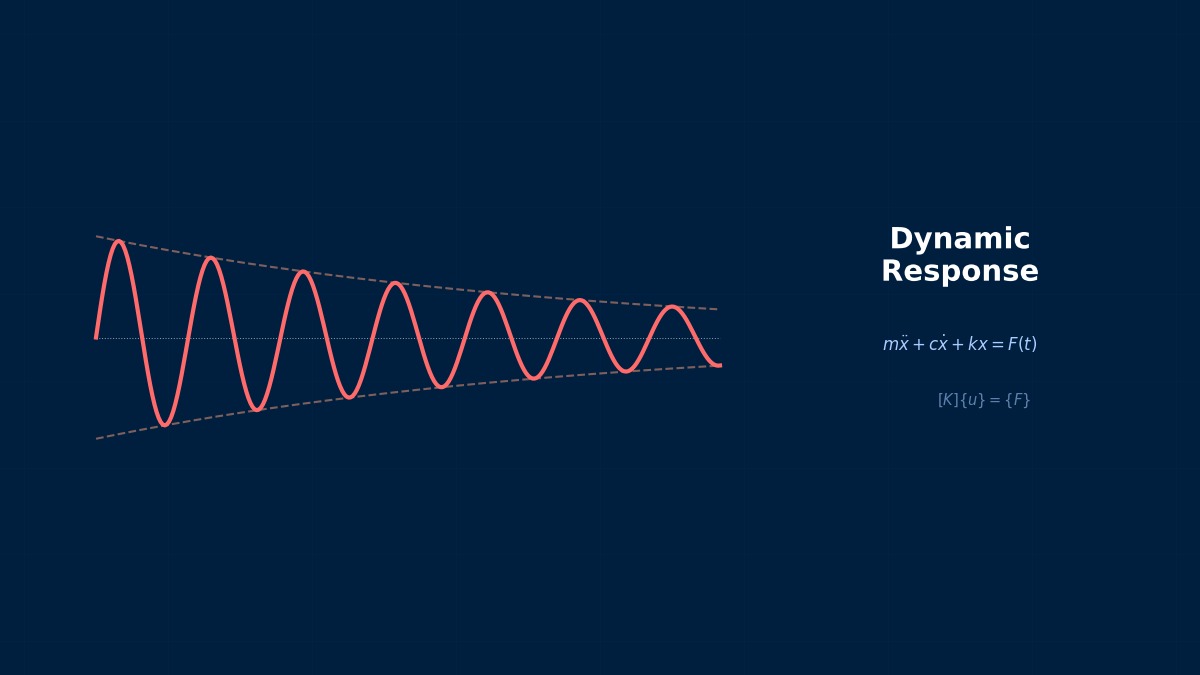
The magnitude of the imbalance force is proportional to $\omega^2$, but the response spikes sharply near resonance.
When the input increase of $\omega^2$ and the amplification of resonance overlap, it results in a very large response. Therefore, avoiding critical speeds (natural frequency = rotational speed) is the top priority design consideration.
Summary
Key Points:
- $F = me\omega^2$ — Imbalance force is proportional to $\omega^2$
- Resonance at Critical Speed — Natural frequency coincides with rotational speed
- ISO 1940 Balance Quality — Specification for allowable imbalance amount
- ISO 10816 Vibration Limits — Allowable values for response vibration
Rotor Imbalance Can Be a Problem Even at the Atomic Level
For ultra-precision spindles (used in semiconductor lithography equipment, exceeding 60,000 rpm), the allowable imbalance amount is below Grade G0.4 (ISO 21940-11), numerically below a few g·mm. This corresponds to a mass eccentricity equivalent to a small piece of paper (approx. 80g/m²) about 1cm² in size. In the 1990s, ASML applied this standard to rotating optical components in EUV lithography machines, becoming a catalyst for tightening the balance standards for precision rotating machinery by one level.
Physical Meaning of Each Term
- Inertia Term (Mass Term): $\rho \ddot{u}$, i.e., "mass × acceleration". Have you ever experienced being thrown forward when braking suddenly? That "feeling of being carried away" is precisely the inertial force. Heavier objects are harder to set in motion and harder to stop once moving. Buildings shake during earthquakes because the ground moves suddenly while the building's mass "gets left behind". In static analysis, this term is set to zero, assuming "forces are applied slowly enough that acceleration can be ignored". It absolutely cannot be omitted in impact loading or vibration problems.
- Stiffness Term (Elastic Restoring Force): $Ku$ or $\nabla \cdot \sigma$. When you pull a spring, you feel a "force trying to return it", right? That's Hooke's law $F=kx$, the essence of the stiffness term. So here's a question—if you pull an iron rod and a rubber band with the same force, which stretches more? Obviously the rubber. This "resistance to stretching" is the Young's modulus $E$, which determines stiffness. A common misconception: "High stiffness = strong" is incorrect. Stiffness is "resistance to deformation", strength is "resistance to failure"—they are different concepts.
- External Force Term (Load Term): Body force $f_b$ (gravity, etc.) and surface force $f_s$ (pressure, contact force, etc.). Think of it this way—the weight of a truck on a bridge is a "force acting on the entire volume" (body force), while the force of the tires pushing on the road is a "force acting only on the surface" (surface force). Wind pressure, water pressure, bolt tightening force... all are external forces. A common mistake here: getting the load direction wrong. Intending "tension" but ending up with "compression"—it sounds like a joke, but it actually happens when coordinate systems are rotated in 3D space.
- Damping Term: Rayleigh damping $C\dot{u} = (\alpha M + \beta K)\dot{u}$. Try plucking a guitar string. Does the sound continue forever? No, it gradually fades away. That's because vibration energy is converted to heat by air resistance and internal friction in the string. Car shock absorbers work on the same principle—they intentionally absorb vibration energy to improve ride comfort. What if damping were zero? Buildings would keep shaking forever after an earthquake. Since that doesn't happen in reality, setting appropriate damping is crucial.
Assumptions and Applicability Limits
- Continuum Assumption: Treats material as a continuous medium, ignoring microscopic heterogeneity.
- Small Deformation Assumption (for linear analysis): Deformation is sufficiently small compared to initial dimensions, and the stress-strain relationship is linear.
- Isotropic Material (unless otherwise specified): Material properties are independent of direction (anisotropic materials require separate tensor definitions).
- Quasi-Static Assumption (for static analysis): Ignores inertial and damping forces, considering only the equilibrium between external and internal forces.
- Non-Applicable Cases: For large deformation/large rotation problems, geometric nonlinearity is required. For nonlinear material behavior like plasticity or creep, constitutive law extensions are needed.
Dimensional Analysis and Unit Systems
| Variable | SI Unit | Notes / Conversion Memo |
|---|---|---|
| Displacement $u$ | m (meter) | When inputting in mm, unify loads and elastic modulus to MPa/N system |
| Stress $\sigma$ | Pa (Pascal) = N/m² | MPa = 10⁶ Pa. Be careful of unit system inconsistency when comparing with yield stress |
| Strain $\varepsilon$ | Dimensionless (m/m) | Note the distinction between engineering strain and logarithmic strain (for large deformation) |
| Elastic Modulus $E$ | Pa | Steel: ~210 GPa, Aluminum: ~70 GPa. Note temperature dependence |
| Density $\rho$ | kg/m³ | In mm system: tonne/mm³ (= 10⁻⁹ tonne/mm³ for steel) |
| Force $F$ | N (Newton) | Unify as N in mm system, N in m system |
Numerical Methods and Implementation
Imbalance Response in FEM
How do you input the imbalance force in FEM?
Nastran
```
$ Imbalance force (rotational speed dependent)
RLOAD2, 100, 200, , , 1.
DLOAD, 300, 1., 1., 100
$ F = meomega^2 → Set force amplitude proportional to ω^2
```
Set the amplitude of RLOAD2 proportional to ω^2 based on imbalance mass and eccentric distance.
Abaqus
```
*STEP
*STEADY STATE DYNAMICS
f1, f2, npoints, 1.
*CLOAD, OP=NEW, AMPLITUDE=unbalance_amp
node, 1, 1.0
node, 2, 1.0
```
Define AMPLITUDE as ω^2. Apply with a 90° phase difference in x and y components (rotating force).
Since the imbalance force rotates, you apply forces with a 90° phase difference in the x and y directions simultaneously, right?
Correct. $F_x = me\omega^2 \cos(\omega t), F_y = me\omega^2 \sin(\omega t)$. In frequency response analysis, input as a complex load $F_x + iF_y$.
Summary
Key Points:
- Input $F = me\omega^2$ as a frequency-dependent load — RLOAD2 (Nastran), AMPLITUDE (Abaqus)
- 90° phase difference in x, y directions — Representation of rotating force
- Coordination with Campbell Diagram — Verification of critical speed avoidance
The Origin of Two-Plane Balancing Dates to 1907
The theory of dynamic two-plane balancing for rotating bodies was formulated by W.E. Dalby in 1907. Today's fully automatic balancing machines (Hofmann, Schenck, etc.) are merely electronic implementations of this two-plane method. The distinction between single-plane and two-plane balancing for automotive tires stems from the mathematical basis in Dalby's theory, which distinguished between "overhung" and "between bearings" cases.
Linear Elements (1st Order Elements)
Linear interpolation between nodes. Low computational cost but low stress accuracy. Beware of shear locking (mitigated by reduced integration or B-bar method).
Quadratic Elements (with Mid-Side Nodes)
Can represent curved deformation. Stress accuracy improves significantly, but degrees of freedom increase by about 2-3 times. Recommended: when stress evaluation is critical.
Full Integration vs Reduced Integration
Full Integration: Risk of over-constraint (locking). Reduced Integration: Risk of hourglass modes (zero-energy modes). Choose appropriately for the situation.
Adaptive Mesh
Automatic refinement based on error indicators (e.g., ZZ estimator). Efficiently improves accuracy in stress concentration areas. Includes h-method (element subdivision) and p-method (order increase).
Newton-Raphson Method
Standard method for nonlinear analysis. Updates the tangent stiffness matrix each iteration. Achieves quadratic convergence within the convergence radius, but computational cost is high.
Modified Newton-Raphson Method
Updates the tangent stiffness matrix using the initial value or every few iterations. Cost per iteration is low, but convergence speed is linear.
Convergence Criteria
Force residual norm: $||R|| / ||F_{ext}|| < \epsilon$ (typically $\epsilon = 10^{-3}$ to $10^{-6}$). Displacement increment norm: $||\Delta u|| / ||u|| < \epsilon$. Energy norm: $\Delta u \cdot R < \epsilon$
Load Increment Method
Instead of applying the full load at once, applies it in small increments. The arc-length method (Riks method) can trace beyond limit points on the load-displacement curve.
Analogy: Direct Method vs Iterative Method
The direct method is like "solving simultaneous equations accurately with pen and paper"—reliable but takes too long for large-scale problems. The iterative method is like "repeatedly guessing to approach the correct answer"—starts with a rough answer but improves accuracy with each iteration. It's the same principle as looking up a word in a dictionary: it's more efficient to open it at an estimated location and adjust forward/backward (iterative) than to search sequentially from the first page (direct).
Relationship Between Mesh Order and Accuracy
1st order elements are like "approximating a curve with a ruler"—represented by straight line segments, so accuracy is limited. 2nd order elements are like a "flexible curve"—can represent curved changes, dramatically improving accuracy even at the same mesh density. However, computational cost per element increases, so judgment should be based on total cost-effectiveness.
Practical Guide
Practical Work for Imbalance Response
What is the practical workflow for imbalance response analysis?
1. Set Imbalance Amount — Calculate $me$ from ISO 1940 G grade × mass
2. Campbell Diagram — Identify critical speeds
3. Imbalance Response Analysis — Displacement, velocity, acceleration at each rotational speed
4. Compare with Vibration Limits — ISO 10816, API 617, etc.
5. If Balancing is Insufficient → Improve balance quality or add damping
ISO 10816 Vibration Limits
| Group | Vibration Velocity (mm/s) rms |
|---|---|
| Good | < 2.8 |
| Acceptable | 2.8 to 7.1 |
| Warning | 7.1 to 18 |
| Unacceptable | > 18 |
So you evaluate based on vibration velocity.
Vibration velocity is proportional to vibration energy, so it correlates well with structural fatigue and bearing life.
Practical Checklist
Jet Engine Balancing is in Units of 0.01g
The fan blades (each about 4kg) of the GE90 engine (for Boeing 777) are adjusted after assembly to have an imbalance of less than 0.01g. Analysis uses MSC Nastran's ROTORDYNAMICS function to calculate imbalance response and confirms the design condition that critical speeds are at least 30% away from each operating point (takeoff, cruise, landing).
Analogy for Analysis Flow
The analysis flow is actually very similar to cooking. First, you buy the ingredients (prepare the CAD model), do the prep work (mesh generation), apply heat (solver execution), and finally plate it (visualization in post-processing). Here's an important question—in cooking, which step is most prone to failure? Actually, it's the "prep work". If mesh quality is poor, the results will be a mess no matter how excellent the solver is.
Pitfalls Beginners Easily Fall Into
Are you checking mesh convergence? Do you think "the calculation ran = the results are correct"? This is actually the most common trap for CAE beginners. The solver provides "some answer" based on the given mesh, but that doesn't guarantee it's the correct physical answer. Always perform a mesh convergence study and verify with simple hand calculations or known results.
Related Topics
なった
詳しく
報告