Modal Frequency Response Analysis
Theory and Physics
What is Frequency Response Analysis?
Professor, what is "Frequency Response Analysis"?
It's an analysis to determine the steady-state response of a structure to a harmonic (sinusoidal) external force. It calculates displacement, acceleration, and stress at each frequency by varying the excitation frequency.
Input: $\{F\} e^{i\omega t}$ (harmonic force with frequency $\omega$)
Output: $\{u\} e^{i\omega t}$ (steady-state response at the same frequency)
So you can see where the resonance peaks are and how large the amplitudes become.
Exactly. The main result is the graph of the FRF (Frequency Response Function) $H(\omega) = u / F$. It shows resonance peaks, anti-resonance valleys, and phase changes.
Mode Method vs. Direct Method
There are two methods for frequency response analysis:
| Method | Principle | Advantages | Disadvantages |
|---|---|---|---|
| Mode Method | Expands in eigenmodes and solves in modal coordinates | Fast. Efficiently calculates many frequency points. | Possible accuracy loss due to insufficient number of modes. |
| Direct Method | Directly solves the system of equations at each frequency | High accuracy. Independent of the number of modes. | High computational cost. Solves for each frequency point. |
The Mode Method uses the results of the natural frequency analysis, right?
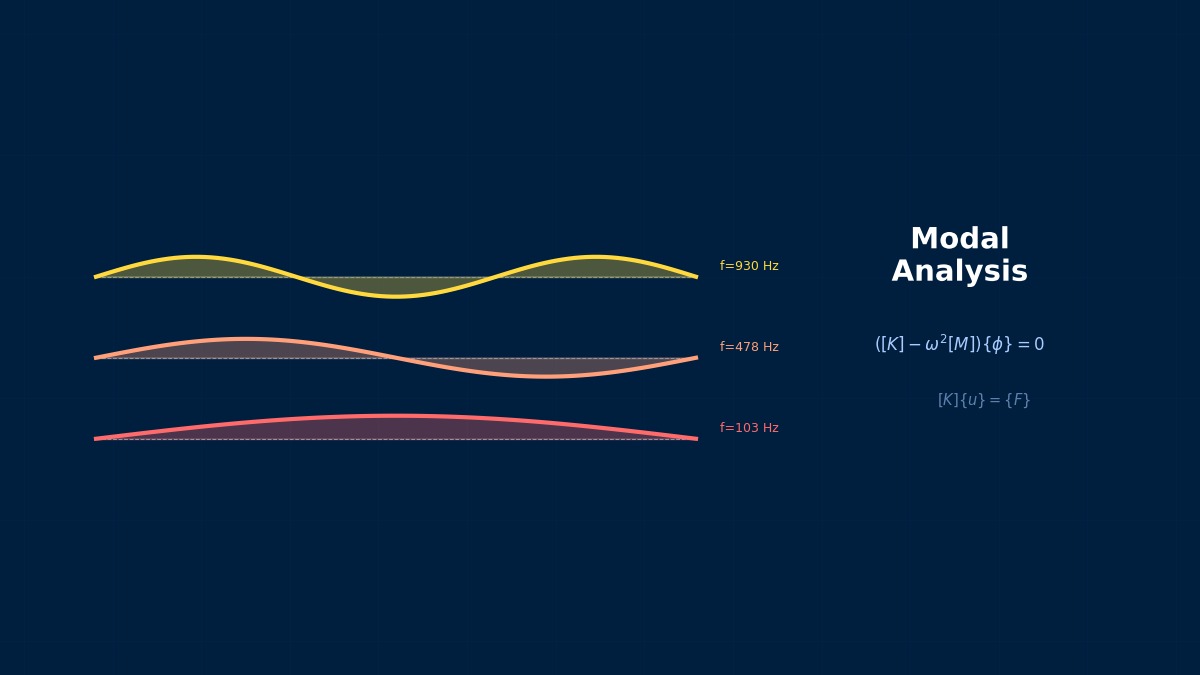
Yes. First, perform an eigenvalue analysis to obtain $N$ modes, then transform the equation of motion into modal coordinates $\{q\}$:
The response of each mode can be solved independently (thanks to modal orthogonality). It's just solving $N$ single-degree-of-freedom systems.
Results of Mode Superposition
Steady-state response in modal coordinates:
Response in physical coordinates:
The denominator has $\omega_i^2 - \omega^2$... resonance occurs when $\omega = \omega_i$ and the denominator approaches zero.
Exactly. The damping term $2i\zeta_i \omega_i \omega$ keeps the amplitude finite at resonance. With $\zeta = 0$ (no damping), the amplitude becomes infinite at resonance.
Nastran
```
SOL 111 $ Mode method frequency response
CEND
METHOD = 10
FREQUENCY = 20
BEGIN BULK
EIGRL, 10, , , 50
FREQ1, 20, 1., 500., 1. $ 1 to 500 Hz, 1 Hz increment
```
Abaqus
```
*STEP
*FREQUENCY
50, ,
*END STEP
*STEP
*STEADY STATE DYNAMICS, DIRECT=NO
1., 500., 500, 1.
*END STEP
```
Ansys
```
/SOLU
ANTYPE, HARMONIC
HROPT, MSUP ! Mode superposition method
HARFRQ, 1., 500.
NSUBST, 500
SOLVE
```
Summary
Let me summarize the mode method frequency response.
Key points:
- Steady-state response to harmonic force — FRF (Frequency Response Function) is the main result.
- Mode Method — Expands in eigenmodes for efficient calculation.
- Resonance peaks occur at $\omega = \omega_i$ — Amplitude is proportional to $1/(2\zeta)$.
- SOL 111 (Nastran), *SSD (Abaqus), HARMONIC MSUP (Ansys)
- Number of modes determines accuracy — Need enough modes to cover 90% effective mass.
So it's a two-step workflow: natural frequency analysis → frequency response analysis.
The natural frequency analysis reveals the "inherent characteristics of the structure," and the frequency response analysis predicts the "response to external forces." This pair forms the basic dynamic analysis workflow.
Mode Superposition is the Same Idea as Fourier Expansion
The mode superposition method represents structural displacement as a linear combination of mode shapes (eigenvectors). Mathematically, this is exactly the same idea as Fourier series expansion. This principle was first applied to structural mechanics by Lord Rayleigh (1877, 'Sound Theory'). Due to the mathematical property that eigenmodes form an orthogonal basis, the N-degree-of-freedom system of equations decomposes into N independent single-degree-of-freedom equations, dramatically speeding up computation.
Physical Meaning of Each Term
- Inertia term (mass term): $\rho \ddot{u}$, i.e., "mass × acceleration". Have you ever experienced being thrown forward when slamming on the brakes? That "feeling of being carried away" is precisely the inertial force. Heavier objects are harder to set in motion and harder to stop once moving. Buildings shake during earthquakes because the ground moves suddenly while the building's mass "gets left behind". In static analysis, this term is set to zero, assuming "forces are applied slowly enough that acceleration is negligible". It absolutely cannot be omitted for impact loads or vibration problems.
- Stiffness term (elastic restoring force): $Ku$ or $\nabla \cdot \sigma$. When you pull a spring, you feel a "force trying to return it", right? That's Hooke's law $F=kx$, the essence of the stiffness term. Now a question—an iron rod and a rubber band, which stretches more under the same force? Obviously the rubber. This "resistance to stretching" is the Young's modulus $E$, which determines stiffness. A common misconception: "high stiffness ≠ strong". Stiffness is "resistance to deformation", strength is "resistance to failure"—different concepts.
- External force term (load term): Body forces $f_b$ (e.g., gravity) and surface forces $f_s$ (pressure, contact forces). Think of it this way—the weight of a truck on a bridge is a "force acting on the entire volume" (body force), while the force of the tires pushing on the road is a "force acting only on the surface" (surface force). Wind pressure, water pressure, bolt tightening force... all are external forces. A common mistake here: getting the load direction wrong. Intending "tension" but it becomes "compression"—sounds like a joke, but it actually happens when coordinate systems are rotated in 3D space.
- Damping term: Rayleigh damping $C\dot{u} = (\alpha M + \beta K)\dot{u}$. Try plucking a guitar string. Does the sound continue forever? No, it gradually fades. That's because vibrational energy is converted to heat by air resistance and internal friction in the string. Car shock absorbers work on the same principle—they intentionally absorb vibrational energy to improve ride comfort. What if damping were zero? Buildings would keep shaking forever after an earthquake. Since that doesn't happen in reality, setting appropriate damping is crucial.
Assumptions and Applicability Limits
- Continuum assumption: Treats material as a continuous medium, ignoring microscopic heterogeneity.
- Small deformation assumption (for linear analysis): Deformation is sufficiently small compared to initial dimensions, and stress-strain relationship is linear.
- Isotropic material (unless specified otherwise): Material properties are independent of direction (anisotropic materials require separate tensor definitions).
- Quasi-static assumption (for static analysis): Ignores inertial and damping forces, considering only equilibrium between external and internal forces.
- Non-applicable cases: For large deformation/large rotation problems, geometric nonlinearity is required. For nonlinear material behavior like plasticity or creep, constitutive law extensions are needed.
Dimensional Analysis and Unit Systems
| Variable | SI Unit | Notes / Conversion Memo |
|---|---|---|
| Displacement $u$ | m (meter) | When inputting in mm, unify loads and elastic modulus to MPa/N system. |
| Stress $\sigma$ | Pa (Pascal) = N/m² | MPa = 10⁶ Pa. Be careful of unit inconsistency when comparing with yield stress. |
| Strain $\varepsilon$ | Dimensionless (m/m) | Note the distinction between engineering strain and logarithmic strain (for large deformations). |
| Elastic modulus $E$ | Pa | Steel: ~210 GPa, Aluminum: ~70 GPa. Note temperature dependence. |
| Density $\rho$ | kg/m³ | In mm system: tonne/mm³ (= 10⁻⁹ tonne/mm³ for steel). |
| Force $F$ | N (Newton) | Unify to N in mm system, N in m system. |
Numerical Methods and Implementation
Computational Efficiency of the Mode Method
Please explain why the Mode Method is faster than the Direct Method.
The Direct Method solves an $n \times n$ (where $n$ = number of DOFs) system of equations at each frequency point. The Mode Method performs one eigenvalue analysis + solves a $N \times N$ (where $N$ = number of modes << $n$) diagonal system at each frequency point.
| Computational Cost | Direct Method | Mode Method |
|---|---|---|
| Per frequency point | $O(n \cdot bw)$ or $O(n^2)$ | $O(N)$ |
| For $M$ frequency points | $M \times O(n \cdot bw)$ | Eigenvalue + $M \times O(N)$ |
With $N = 100$ modes and $n = 1{,}000{,}000$ DOFs, the Mode Method is 10,000 times faster!
That's why the Mode Method is overwhelmingly advantageous for cases like NVH analysis that require calculating many frequency points (500~1000 points).
Importance of Residual Modes
What about the influence of higher-order modes that are not included?
Corrected with Residual Modes (Residual Vectors). Approximates the contribution of higher-order modes using static force-displacement relationships. Automatically added in Nastran with RESVEC=YES.
Without residual modes, do results deviate at low frequencies?
Not at low frequencies, but at high frequencies (near the upper limit of the range of interest). Residual modes correct the "truncation error of the modal expansion". In practice, RESVEC should always be enabled.
FRF Output
Main types of FRF (Frequency Response Function):
| FRF Type | Definition | Usage |
|---|---|---|
| Compliance | $u/F$ | Displacement response |
| Mobility | $v/F = i\omega \cdot u/F$ | Velocity response |
| Inertance | $a/F = -\omega^2 \cdot u/F$ | Acceleration response |
Which one is used in experiments?
In experimental modal analysis, inertance (acceleration/force) is common because accelerometers are most widely used. When comparing FEM results with experiments, output in the same format.
Summary
Let me summarize the numerical methods for mode method frequency response.
Key points:
- The Mode Method is overwhelmingly faster than the Direct Method — Advantageous for many frequency points.
- Correct higher-order effects with Residual Modes (RESVEC) — Should always be enabled.
- FRF format —
Related Topics
Structural直接法周波数応答解析StructuralModal Transient Response Analysis用語集周波数応答解析 — CAE用語解説StructuralFrequency Sweep and Resonance EvaluationStructuralPower Spectral Density Response AnalysisStructuralVibration Test Simulationこの記事の評価ご回答ありがとうございます!参考に
なったもっと
詳しく誤りを
報告