Natural Frequency Analysis
Natural Frequency Analysis: Theoretical Foundations
What is Natural Frequency?
Professor, what is "natural frequency"?
It is the natural vibration frequency of a structure when it vibrates without any external force. All structures have their own natural frequency, and when the frequency of an external force matches this, resonance occurs.
What's the problem with resonance?
During resonance, the amplitude increases rapidly. Bridge collapses (Tacoma Narrows Bridge, 1940), building damage (during earthquakes), machine failures (dangerous speeds of rotating bodies)... all are caused by resonance. Understanding the natural frequency is the most basic requirement of structural design.
Governing Equation
Equation for undamped free vibration:
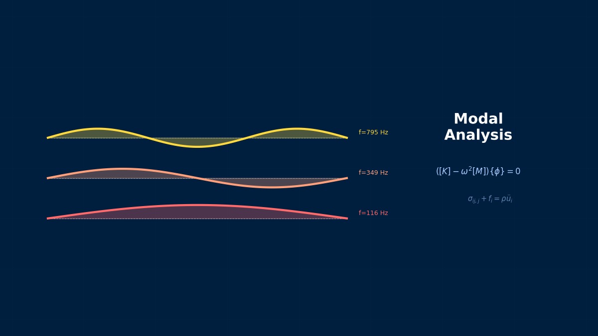
Assuming a solution of $\{u\} = \{\phi\} e^{i\omega t}$, we get the eigenvalue problem:
It has the same form as the buckling analysis equation $([K] + \lambda [K_\sigma])\{\phi\} = \{0\}$!
Exactly the same mathematical structure. In buckling, $[M]$ takes the place of $[K_\sigma]$. Therefore, the same eigenvalue solver (Lanczos method, etc.) can be used.
$\omega_i$ is the angular frequency (rad/s), $f_i = \omega_i / (2\pi)$ is the natural frequency (Hz), and $\{\phi_i\}$ is the mode shape.
Natural Frequency of a Single-Degree-of-Freedom System
Before FEM, the most basic case:
It's determined solely by the spring constant $k$ and mass $m$. Higher stiffness and smaller mass lead to higher frequency.
This simple relationship is very useful for sanity checking FEM results. Estimate the equivalent stiffness and equivalent mass of the structure to get an order-of-magnitude estimate for $f$.
Natural Frequency of Beams
Fundamental (first) natural frequency of basic beams:
| Condition | $f_1$ | Note |
|---|---|---|
| Cantilever Beam | $\frac{3.516}{2\pi L^2}\sqrt{\frac{EI}{\rho A}}$ | Lowest |
| Simply Supported Beam | $\frac{\pi^2}{2\pi L^2}\sqrt{\frac{EI}{\rho A}}$ | |
| Fixed-Fixed Beam | $\frac{22.37}{2\pi L^2}\sqrt{\frac{EI}{\rho A}}$ | Highest |
The natural frequency changes quite a bit depending on the boundary conditions.
There's a difference of over 6 times between cantilever and fixed-fixed. If FEM results deviate significantly from theoretical values, the boundary condition settings should be the first thing to suspect.
Natural Frequency Analysis in FEM
What is the procedure for finding natural frequencies with FEM?
1. Modeling — Mesh, material ($E, \rho$), boundary conditions
2. Execute Eigenvalue Analysis — Use Lanczos method to find the lower $n$ modes
3. Check Results — Natural frequencies and mode shapes
4. Verification — Compare with theoretical solutions or experimental modal analysis
Unlike static analysis, the material constant $\rho$ (density) is required here.
Correct. Static analysis only needs $E$, but natural frequency analysis requires $\rho$. Forgetting to set the density will result in natural frequencies being zero or infinite. This is a very common mistake.
Summary
Let me organize the theory of natural frequency analysis.
Key points:
- $([K] - \omega^2 [M])\{\phi\} = \{0\}$ — Same eigenvalue problem as buckling
- $f = (1/2\pi)\sqrt{k/m}$ — The foundation of everything. Use it for sanity checks
- Boundary conditions significantly change natural frequency — 6x difference between cantilever vs. fixed-fixed
- Density $\rho$ setting is mandatory — Results become meaningless if forgotten
- Avoiding resonance is the design goal — Separate the external force frequency from the natural frequency
So natural frequency analysis is the most basic dynamic analysis to know "at what Hz a structure vibrates".
Exactly. Natural frequency analysis is the foundation for all dynamic analyses (response analysis, time history analysis). Dynamic design cannot be established without it.
From Hooke's Law to Vibration Theory
Robert Hooke published the proportional relationship between elastic force and displacement (Hooke's law) in 1678, but he himself did not reach the theory of vibration frequency. It was Christian Huygens who completed it, deriving the period formula for a simple pendulum T=2π√(L/g) from its isochronism in 1673. This formula is a special case of the current single-degree-of-freedom frequency formula fn=1/(2π)√(k/m), a fundamental equation that has remained unchanged for over 300 years.
Computational Methods for Natural Frequency Analysis
Eigenvalue Solver
How is the eigenvalue problem for natural frequencies solved?
The same solver used for buckling analysis can be used. The Lanczos method is the industry standard.
| Method | Characteristics | Application |
|---|---|---|
| Lanczos Method | Optimal for large-scale sparse matrices. Efficiently extracts lower modes | Industry standard |
| Subspace Iteration Method | More stable than Lanczos but slower | Closely spaced eigenvalues |
| AMLS (Automated Multi-Level Substructuring) | Handles extremely large-scale problems | Millions of DOF |
What is AMLS?
AMLS is Nastran's large-scale eigenvalue analysis method. It automatically partitions the structure into substructures, finds the eigenvalues of each substructure individually, and then assembles the whole. It can efficiently find hundreds of modes for models with millions of DOF.
Nastran
```
SOL 103
CEND
METHOD = 10
BEGIN BULK
EIGRL, 10, , , 20 $ Find 20 modes
```
Abaqus
```
*STEP
*FREQUENCY, EIGENSOLVER=LANCZOS
20, ,
*END STEP
```
Ansys
```
/SOLU
ANTYPE, MODAL
MODOPT, LANB, 20 ! 20 modes using Lanczos method
SOLVE
```
The Lanczos method is the default in all solvers.
In modern FEM solvers, it's fair to say that eigenvalue analysis = Lanczos method. The setting is simply specifying "the number of modes to find".
Mass Matrix Selection
Which should we use, consistent mass or lumped mass?
The accuracy of natural frequencies depends on the mass matrix:
- Consistent mass — High accuracy. Recommended default
- Lumped mass — Faster computation but slightly lower accuracy. Differences appear in higher modes
The default for Nastran and Abaqus is consistent mass.