Miner則(累積損傷則)

Category: 構造解析 | Integrated 2026-04-06
CAE visualization for miners rule theory - technical simulation diagram
Miner則(累積損傷則)

Theory and Physics

What is Miner's Rule?

🧑‍🎓

Professor, please teach me about Miner's Rule (the cumulative damage rule).


🎓

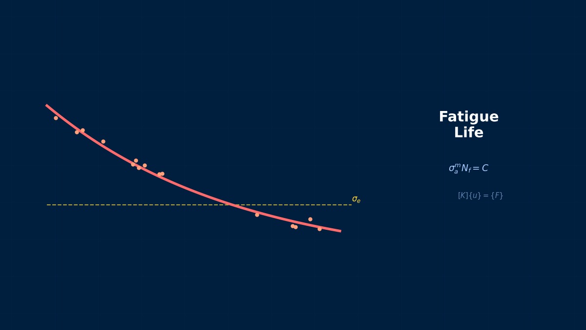
Palmgren-Miner's Rule (1945) evaluates cumulative fatigue damage under variable loading. Failure occurs when the sum of the damage ratios at each stress level reaches 1:


$$ D = \sum_{i=1}^{k} \frac{n_i}{N_i} = 1 $$

$n_i$ is the actual number of cycles at stress level $i$, $N_i$ is the S-N life at that stress level. Failure at $D = 1$.


🧑‍🎓

It's just summing up the "consumption rate" for each level. So simple.


🎓

It's simple but has the problem of ignoring the load sequence effect. Life changes depending on whether the order is high stress → low stress or the reverse, but Miner's Rule does not capture this effect. Still, it's the standard in practice.


Summary

🎓
  • Failure at $D = \sum n_i/N_i = 1$ — Linear cumulative damage
  • Ignores load sequence effect — Can be non-conservative
  • Standard in practice — Simple and widely applicable
  • In design, use $D < 1/SF$ (Safety Factor) — $D < 0.5$ is common

  • Coffee Break Yomoyama Talk

    The "Mysterious 1.0" of Miner's Rule

    The linear cumulative damage rule (Miner's rule) predicts failure when the damage sum reaches 1.0, but actual failure scatters between 0.3 and 3.0. This was a limitation Miner himself acknowledged when he published it in 1945. The main cause is the sequence effect: damage accumulates faster when large amplitude loads are applied first, and slower when the order is small → large.

    Physical Meaning of Each Term
    • Inertia Term (Mass Term): $\rho \ddot{u}$, i.e., "mass × acceleration". Have you ever experienced being thrown forward when slamming on the brakes? That "feeling of being pulled" is precisely the inertial force. Heavier objects are harder to set in motion and harder to stop once moving. Buildings shake during earthquakes because the ground moves suddenly while the building's mass "gets left behind". In static analysis, this term is set to zero, assuming "forces are applied slowly enough that acceleration is negligible". It absolutely cannot be omitted in impact loads or vibration problems.
    • Stiffness Term (Elastic Restoring Force): $Ku$ or $\nabla \cdot \sigma$. When you stretch a spring, you feel a "force trying to return it", right? That's Hooke's law $F=kx$, the essence of the stiffness term. Here's a question—if you pull an iron rod and a rubber band with the same force, which stretches more? Obviously the rubber band. This "resistance to stretching" is the Young's modulus $E$, which determines stiffness. A common misconception: "High stiffness ≠ strong". Stiffness is "resistance to deformation", strength is "resistance to failure"—different concepts.
    • External Force Term (Load Term): Body forces $f_b$ (gravity, etc.) and surface forces $f_s$ (pressure, contact forces, etc.). Think of it this way—the weight of a truck on a bridge is a "force acting on the entire contents" (body force), the force of the tires pushing on the road surface is a "force acting only on the surface" (surface force). Wind pressure, water pressure, bolt tightening force... all are external forces. A typical mistake here: getting the load direction wrong. Intending "tension" but it becomes "compression"—sounds like a joke, but it actually happens when coordinate systems are rotated in 3D space.
    • Damping Term: Rayleigh damping $C\dot{u} = (\alpha M + \beta K)\dot{u}$. Try plucking a guitar string. Does the sound continue forever? No, it gradually fades. That's because vibration energy is converted to heat by air resistance and internal friction in the string. Car shock absorbers work on the same principle—they intentionally absorb vibration energy to improve ride comfort. What if damping were zero? Buildings would keep swaying forever after an earthquake. Since that doesn't happen in reality, setting appropriate damping is crucial.
    Assumptions and Applicability Limits
    • Continuum assumption: Treats material as a continuous medium, ignoring microscopic inhomogeneity.
    • Small deformation assumption (for linear analysis): Deformation is sufficiently small compared to initial dimensions, stress-strain relationship is linear.
    • Isotropic material (unless otherwise specified): Material properties are independent of direction (anisotropic materials require separate tensor definitions).
    • Quasi-static assumption (for static analysis): Ignores inertial and damping forces, considers only equilibrium between external and internal forces.
    • Non-applicable cases: Large deformation/large rotation problems require geometric nonlinearity. Nonlinear material behavior like plasticity or creep requires constitutive law extensions.
    Dimensional Analysis and Unit Systems
    VariableSI UnitNotes / Conversion Memo
    Displacement $u$m (meter)When inputting in mm, unify loads and elastic modulus to MPa/N system.
    Stress $\sigma$Pa (Pascal) = N/m²MPa = 10⁶ Pa. Be careful of unit inconsistency when comparing with yield stress.
    Strain $\varepsilon$Dimensionless (m/m)Note the distinction between engineering strain and logarithmic strain (for large deformation).
    Elastic modulus $E$PaSteel: ~210 GPa, Aluminum: ~70 GPa. Note temperature dependence.
    Density $\rho$kg/m³In mm system: tonne/mm³ (= 10⁻⁹ tonne/mm³ for steel).
    Force $F$N (Newton)Unify as N in mm system, N in m system.

    Numerical Methods and Implementation

    Miner's Rule in FEM

    🎓

    1. FEM stress → Rainflow method for cycle extraction → S-N life $N_i$ for each $\Delta\sigma_i$ → $D = \sum n_i/N_i$


    Automatically calculated in all fatigue software (nCode, fe-safe, FEMFAT).


    Summary

    🎓
    • Rainflow → S-N → Miner's Rule — Standard flow for variable amplitude fatigue
    • Automatically calculated in all fatigue software

    • Coffee Break Yomoyama Talk

      The Key is Combination with the Rainflow Method

      To use Miner's rule in practice, cycles are extracted from irregular load time histories using the rainflow method, the life Ni on the S-N curve for each amplitude is read, and the damage Σ(ni/Ni) is calculated. Since the 1990s, automotive manufacturers have developed in-house software to automatically process measurement data, enabling fatigue damage evaluation of 1 minute of actual driving data within 5 minutes.

      Linear Elements (1st Order Elements)

      Linear interpolation between nodes. Low computational cost but low stress accuracy. Beware of shear locking (mitigated by reduced integration or B-bar method).

      Quadratic Elements (with Mid-side Nodes)

      Can represent curved deformation. Stress accuracy improves significantly, but degrees of freedom increase by about 2-3 times. Recommended: when stress evaluation is critical.

      Full Integration vs Reduced Integration

      Full Integration: Risk of over-constraint (locking). Reduced Integration: Risk of hourglass modes (zero-energy modes). Choose appropriately for the situation.

      Adaptive Mesh

      Automatic refinement based on error indicators (e.g., ZZ estimator). Efficiently improves accuracy in stress concentration areas. Includes h-method (element subdivision) and p-method (order increase).

      Newton-Raphson Method

      Standard method for nonlinear analysis. Updates the tangent stiffness matrix each iteration. Quadratic convergence within the convergence radius, but high computational cost.

      Modified Newton-Raphson Method

      Updates the tangent stiffness matrix using the initial value or every few iterations. Cost per iteration is low, but convergence speed is linear.

      Convergence Criteria

      Force residual norm: $||R|| / ||F_{ext}|| < \epsilon$ (typically $\epsilon = 10^{-3}$ to $10^{-6}$). Displacement increment norm: $||\Delta u|| / ||u|| < \epsilon$. Energy norm: $\Delta u \cdot R < \epsilon$

      Load Increment Method

      Instead of applying the full load at once, apply it in small increments. The arc-length method (Riks method) can trace beyond extremum points on the load-displacement relationship.

      Analogy: Direct Method vs Iterative Method

      The direct method is like "solving simultaneous equations accurately with pen and paper"—reliable but takes too long for large-scale problems. The iterative method is like "repeatedly guessing to approach the correct answer"—starts with a rough answer but accuracy improves with each iteration. It's the same principle as looking up a word in a dictionary: it's more efficient to estimate where to open it and adjust forward/backward (iterative method) than to search sequentially from the first page (direct method).

      Relationship Between Mesh Order and Accuracy

      1st order elements are like "approximating a curve with a ruler"—represented by straight line segments, so accuracy is limited. 2nd order elements are like "flexible curves"—can represent curved changes, dramatically improving accuracy even at the same mesh density. However, computational cost per element increases, so judge based on overall cost-effectiveness.

      Practical Guide

      Miner's Rule in Practice

      🎓

      Used in all variable amplitude fatigue.


      Practical Checklist

      🎓
      • [ ] Are cycles correctly extracted by the rainflow method?
      • [ ] Is the S-N curve correct?
      • [ ] Include contribution of cycles below the fatigue limit? (e.g., Haibach modification)
      • [ ] Confirm $D < 1/SF$ (Safety Factor)
      • [ ] Identify critical locations using $D$ contour plots

      • Coffee Break Yomoyama Talk

        Example: Fatigue Life Evaluation of a Truck Axle

        In actual truck axle design, the standard load spectrum from Japanese Industrial Standard JASO M 305 is combined with Miner's rule. For a 10-ton capacity vehicle, 10,000 km of driving corresponds to about 5 million cycles. Using load ratios of 3:5:2 for empty, fully loaded, and bump crossing, a design equivalent to a 1 million km life is possible.

        Analogy: Analysis Flow

        The analysis flow is actually very similar to cooking. First, buy ingredients (prepare CAD model), do the prep work (mesh generation), apply heat (solver execution), and finally plate it (post-processing visualization). Here's an important question—which step in cooking is most prone to failure? Actually, it's "prep work". If mesh quality is poor, the results will be a mess no matter how good the solver is.

        Pitfalls Beginners Often Fall Into

        Are you checking mesh convergence? Do you think "the calculation ran = the result is correct"? This is actually the most common trap for CAE beginners. The solver will always return "some answer" for the given mesh. But if the mesh is too coarse, that answer is far from reality. Confirm that results stabilize with at least three levels of mesh density—neglecting this leads to the dangerous assumption that "the computer gave the answer, so it must be correct".

        Thinking About Boundary Conditions

        Setting boundary conditions is like "writing the problem statement" for an exam. If the problem statement is wrong? No matter how accurately you calculate, the answer will be wrong. "Is this surface really fully fixed?" "Is this load really uniformly distributed?"—Correctly modeling real-world constraints is actually the most important step in the entire analysis.

        Software Comparison

        Tools

        🎓

        Standard in all fatigue software. nCode, fe-safe, FEMFAT, Ansys Fatigue Tool.


        Coffee Break Yomoyama Talk

        Differences in Miner's Rule Implementation Among Solver Vendors

        In ABAQUS, ANSYS, and MSC Nastran, the default critical value for the linear cumulative damage rule (Miner's rule) is D=1.0, which is common. However, Simulia fe-safe recommends D=0.5 as the default, adopting a conservative setting aligned with the aerospace AS9100 standard. In practice, even with the same FE model, the allowable number of cycles can vary by a factor of 2 depending on solver choice.

        The Three Most Important Questions for Selection

        • "What to solve?": Does it support the physical models/element types needed for Miner's Rule (cumulative damage rule)? For example, in fluids, the presence of LES support; in structures, the ability to handle contact/large deformation makes a difference.
        • "Who will use it?": For beginner teams, tools with rich GUIs are suitable; for experienced users, flexible script-driven tools are better. Similar to the difference between automatic (GUI) and manual (script) transmission cars.
        • "How far to expand?": Selection considering future expansion of analysis scale (HPC support), deployment to other departments, and integration with other tools leads to long-term cost reduction.

        Advanced Technology

        Advanced Topics in Miner's Rule

        🎓
        • Nonlinear Miner's Rule — Modified Miner's rule including load sequence effects
        • Probabilistic Miner's Rule — Statistical evaluation of the distribution of $D$
        • Miner's Rule + Crack Growth — Integration of crack nucleation (Miner) + crack propagation (Paris' Law)

        • Coffee Break Yomoyama Talk
          関連シミュレーター

          この分野のインタラクティブシミュレーターで理論を体感しよう

          シミュレーター一覧

          関連する分野

          この記事の評価
          ご回答ありがとうございます!
          参考に
          なった
          もっと
          詳しく
          誤りを
          報告
          参考になった
          0
          もっと詳しく
          0
          誤りを報告
          0
          Written by NovaSolver Contributors
          Anonymous Engineers & AI — サイトマップ