Concrete Damaged Plasticity Model (CDP)

Category: 構造解析 | Integrated 2026-04-06
CAE visualization for concrete damaged theory - technical simulation diagram
損傷塑性コンクリートモデル(CDP)

Theory and Physics

What is the CDP Model?

🧑‍🎓

Professor, what is the CDP model?


🎓

CDP (Concrete Damaged Plasticity) is a constitutive model for concrete in Abaqus. It is a combination of Plasticity (based on DP criterion) + Damage (tensile cracking + compressive crushing).


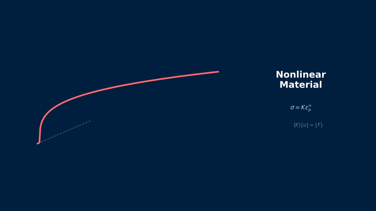
Special Characteristics of Concrete

🎓
  • Tensile strength is 1/10 of compressive strength — Weak in tension
  • Softening in tension (cracking) — Tensile stress decreases after peak
  • Softening also in compression — Stress decreases after peak compressive strength
  • Tension-compression asymmetry — Recovery after tensile damage under compression (stiffness recovery)

  • CDP Composition

    🎓
    • Yield surface — Modified Drucker-Prager. Tension-compression asymmetry
    • Tensile damage — Cracking in tension → stiffness reduction
    • Compressive damage — Crushing in compression → stiffness reduction
    • Stiffness recovery — Compressive stiffness recovers when tensile cracks close

    • Settings in FEM

      🎓

      ```

      *CONCRETE DAMAGED PLASTICITY

      dilation_angle, eccentricity, fb0/fc0, K, viscosity

      *CONCRETE COMPRESSION HARDENING

      stress, inelastic_strain

      *CONCRETE TENSION STIFFENING

      stress, cracking_strain

      *CONCRETE COMPRESSION DAMAGE

      damage, inelastic_strain

      *CONCRETE TENSION DAMAGE

      damage, cracking_strain

      ```


      Summary

      🎓

      Key Points:


      • CDP = Drucker-Prager plasticity + Tensile/Compressive damage — Dedicated to concrete
      • Tensile softening (cracking) + Compressive softening (crushing) — Special behavior of concrete
      • Stiffness recovery — Recovery under compression when tensile cracks close
      • Abaqus CDP is the de facto standard in research

      Coffee Break Coffee Break Talk

      The Two Fathers of the CDP Model

      The Concrete Damaged Plasticity (CDP) model originates from the 1989 paper "A plastic-damage model for concrete" by J. Lubliner and J. Oliver (Universitat Politècnica de Catalunya). Later in 1998, Lee & Fenves from the Abaqus team significantly improved the numerical stability of strain softening, leading to the formulation now most widely used worldwide. This Lee-Fenves version was commercialized as Concrete Damaged Plasticity in Abaqus/Standard.

      Physical Meaning of Each Term
      • Inertia term (mass term): $\rho \ddot{u}$, meaning "mass × acceleration". Have you ever experienced being thrown forward when slamming on the brakes? That "feeling of being carried forward" is precisely the inertial force. Heavier objects are harder to set in motion and harder to stop once moving. Buildings shake during earthquakes because the ground moves suddenly while the building's mass "gets left behind". In static analysis, this term is set to zero, assuming "forces are applied slowly so acceleration can be ignored". It cannot be omitted in impact loads or vibration problems.
      • Stiffness term (elastic restoring force): $Ku$ or $\nabla \cdot \sigma$. When you pull a spring, you feel a "force trying to return it", right? That's Hooke's law $F=kx$, the essence of the stiffness term. So a question—if you pull an iron rod and a rubber band with the same force, which stretches more? Obviously the rubber band. This "resistance to stretching" is the Young's modulus $E$, which determines stiffness. A common misconception: "high stiffness ≠ strong". Stiffness is "resistance to deformation", strength is "resistance to failure"—they are different concepts.
      • External force term (load term): Body force $f_b$ (gravity, etc.) and surface force $f_s$ (pressure, contact force, etc.). Think of it this way—the weight of a truck on a bridge is a "force acting on the entire volume" (body force), while the force of the tires pushing on the road surface is a "force acting only on the surface" (surface force). Wind pressure, water pressure, bolt tightening force... all are external forces. A typical pitfall here: getting the load direction wrong. Intending "tension" but it becomes "compression"—sounds like a joke, but it actually happens when coordinate systems are rotated in 3D space.
      • Damping term: Rayleigh damping $C\dot{u} = (\alpha M + \beta K)\dot{u}$. Try plucking a guitar string. Does the sound continue forever? No, it gradually fades away. That's because vibration energy is converted to heat by air resistance and internal friction in the string. Car shock absorbers work on the same principle—they intentionally absorb vibration energy to improve ride comfort. What if damping were zero? Buildings would keep shaking forever after an earthquake. Since that doesn't happen in reality, setting appropriate damping is crucial.
      Assumptions and Applicability Limits
      • Continuum assumption: Treats material as a continuous medium, ignoring microscopic heterogeneity.
      • Small deformation assumption (for linear analysis): Deformation is sufficiently small compared to initial dimensions, and stress-strain relationship is linear.
      • Isotropic material (unless specified otherwise): Material properties are independent of direction (anisotropic materials require separate tensor definitions).
      • Quasi-static assumption (for static analysis): Ignores inertial and damping forces, considering only equilibrium between external and internal forces.
      • Non-applicable cases: Large deformation/large rotation problems require geometric nonlinearity. Nonlinear material behavior like plasticity or creep requires constitutive law extensions.
      Dimensional Analysis and Unit Systems
      VariableSI UnitNotes / Conversion Memo
      Displacement $u$m (meter)When inputting in mm, unify loads and elastic modulus to MPa/N system.
      Stress $\sigma$Pa (Pascal) = N/m²MPa = 10⁶ Pa. Be careful of unit system inconsistency when comparing with yield stress.
      Strain $\varepsilon$Dimensionless (m/m)Note the distinction between engineering strain and logarithmic strain (for large deformation).
      Elastic modulus $E$PaSteel: ~210 GPa, Aluminum: ~70 GPa. Note temperature dependence.
      Density $\rho$kg/m³In mm system: tonne/mm³ (= 10⁻⁹ tonne/mm³ for steel).
      Force $F$N (Newton)Unify as N in mm system, N in m system.

      Numerical Methods and Implementation

      CDP Parameters

      🎓
      ParameterTypical ValueMeaning
      Dilation angle ($\psi$)30–40°Dilatancy angle
      Eccentricity0.1Eccentricity of the hyperbola
      $f_{b0}/f_{c0}$1.16Biaxial/uniaxial compressive strength ratio
      $K$2/3Yield surface shape parameter
      Viscosity0.0001–0.001Viscosity regularization
      🧑‍🎓

      Why is viscosity regularization (Viscosity) necessary?


      🎓

      Concrete tensile softening has strong mesh dependency. Viscosity regularization "smoothes out" localization to improve convergence. $\mu = 10^{-4} \sim 10^{-3}$ is typical. Too large makes the response inaccurate.


      Summary

      🎓
      • 5 plasticity parameters + Compression/tension hardening curves + Damage variables
      • Viscosity regularization improves convergence — $\mu = 10^{-4}$
      • Abaqus CDP has the most track record — Nonlinear analysis of RC structures

      • Coffee Break Coffee Break Talk

        Tensile Strength is Only 1/10 of Compression

        Ordinary concrete compressive strength is generally 24–60 N/mm², but its tensile strength is only about 1/10 of that, at 2–5 N/mm². The CDP model expresses this extreme asymmetry with independent damage variables for tension and compression (d_t, d_c). In FEM analysis, the input of the tensile stress-strain relationship most sensitively affects the final results, so the accuracy of the tensile softening curve setting determines the analysis quality.

        Linear Elements (1st-order elements)

        Linear interpolation between nodes. Low computational cost but low stress accuracy. Beware of shear locking (mitigated by reduced integration or B-bar method).

        Quadratic Elements (with mid-side nodes)

        Can represent curved deformation. Stress accuracy improves significantly, but degrees of freedom increase by about 2–3 times. Recommended: when stress evaluation is important.

        Full integration vs Reduced integration

        Full integration: Risk of over-constraint (locking). Reduced integration: Risk of hourglass modes (zero-energy modes). Choose appropriately for the situation.

        Adaptive Mesh

        Automatic refinement based on error indicators (e.g., ZZ estimator). Efficiently improves accuracy in stress concentration areas. Includes h-method (element subdivision) and p-method (order increase).

        Newton-Raphson Method

        Standard method for nonlinear analysis. Updates tangent stiffness matrix every iteration. Achieves quadratic convergence within convergence radius, but computational cost is high.

        Modified Newton-Raphson Method

        Updates tangent stiffness matrix using initial value or every few iterations. Cost per iteration is low, but convergence speed is linear.

        Convergence Criteria

        Force residual norm: $||R|| / ||F_{ext}|| < \epsilon$ (typically $\epsilon = 10^{-3}$–$10^{-6}$). Displacement increment norm: $||\Delta u|| / ||u|| < \epsilon$. Energy norm: $\Delta u \cdot R < \epsilon$

        Load Increment Method

        Applies total load in small increments rather than all at once. The arc-length method (Riks method) can trace beyond limit points on the load-displacement curve.

        Analogy: Direct Method vs Iterative Method

        The direct method is like "solving simultaneous equations accurately with pen and paper"—reliable but takes too long for large-scale problems. The iterative method is like "repeatedly guessing to approach the correct answer"—starts with a rough answer but improves accuracy with each iteration. It's the same principle as looking up a word in a dictionary: it's more efficient to estimate where to open it and adjust forward/backward (iterative method) than to search sequentially from the first page (direct method).

        Relationship Between Mesh Order and Accuracy

        1st-order elements are like "approximating a curve with a ruler"—represented by straight line segments, so accuracy is limited. 2nd-order elements are like "flexible curves"—can represent curved changes, dramatically improving accuracy even at the same mesh density. However, computational cost per element increases, so judge based on total cost-effectiveness.

        Practical Guide

        CDP in Practice

        🎓

        Used for seismic analysis of RC buildings, concrete dams, nuclear containment vessels, detailed analysis of PCa members.


        Practical Checklist

        🎓
        • [ ] Is the compression hardening curve based on material tests (cylinder compression test)?
        • [ ] Is the tensile softening based on fracture energy $G_f$?
        • [ ] Have you confirmed that the viscosity regularization parameter $\mu$ does not affect the results?
        • [ ] Are reinforcing bars correctly modeled as embedded elements?
        • [ ] Does the mesh size align with the characteristic length of tensile softening?

        • Coffee Break Coffee Break Talk

          The Great East Japan Earthquake and Seismic Analysis

          After the 2011 Great East Japan Earthquake, FEM analysis using the CDP model was utilized to evaluate the seismic performance of many existing RC buildings. In commissioned research by the Ministry of Land, Infrastructure, Transport and Tourism (2012–2014), it was confirmed that the maximum load prediction by static incremental analysis (pushover analysis) using the CDP model fell within ±15% of loading test values, and it was officially recognized as a complementary method for seismic diagnosis of existing buildings.

          Analogy of the Analysis Flow

          The analysis flow is actually very similar to cooking. First, buy the ingredients (prepare CAD model), do the prep work (mesh generation), apply heat (solver execution), and finally plate it (visualization in post-processing). Here's an important question—which step in cooking is most prone to failure? Actually, it's the "prep work". If mesh quality is poor, the results will be a mess no matter how good the solver is.

          Pitfalls Beginners Often Fall Into

          Are you checking mesh convergence? Do you think "the calculation ran = the result is correct"? This is actually the most common trap for CAE beginners. The solver will always return "some answer" for the given mesh. But if the mesh is too coarse, that answer is far from reality. Confirm that results stabilize with at least three levels of mesh density—neglecting this leads to the dangerous assumption that "the computer gave the answer, so it must be correct".

          Thinking About Boundary Conditions

          Setting boundary conditions is the same as "writing the problem statement" for an exam. If the problem statement is wrong? No matter how accurately you calculate, the answer will be wrong. "Is this surface really fully fixed?" "Is this load really uniformly distributed?"—Correctly modeling real-world constraint conditions is actually the most important step in the entire analysis.

          Software Comparison

          CDP Tools

          🎓
          • Abaqus CDP — De facto standard in research. Most cited in papers.
          • Ansys — William-Warnke / SOLID65. Older but proven.
          • ATENA — Concrete-specific FEM. Detailed analysis of RC structures.
          • DIANA — Concrete + geotechnical-specific FEM.
          • LS-DYNAMAT_072R3 (KCC), MAT_159 (CSCM)

          • Selection Guide

            🎓
            • RC structure researchAbaqus CDP
            • RC structure practical work → ATENA or DIANA (concrete-specific)
            • Concrete failure under impactLS-DYNA KCC/CSCM

            • Coffee Break Coffee Break Talk

              Implementation Differences Between Midas and Abaqus

              The CDP model is also implemented in Midas FEA NX, LS-DYNA (MAT_CDPM), and OpenSees (Concrete07) besides Abaqus. However, the yield function forms differ slightly; Abaqus uses a hyperbolic Drucker-Prager...

              関連シミュレーター

              この分野のインタラクティブシミュレーターで理論を体感しよう

              シミュレーター一覧

              関連する分野

              熱解析製造プロセス解析V&V・品質保証
              この記事の評価
              ご回答ありがとうございます!
              参考に
              なった
              もっと
              詳しく
              誤りを
              報告
              参考になった
              0
              もっと詳しく
              0
              誤りを報告
              0
              Written by NovaSolver Contributors
              Anonymous Engineers & AI — サイトマップ
              About the Authors