Solve v = v₀ + at, visualize projectile arcs, and sketch v-t graphs to instantly see the corresponding x-t and a-t curves. From high school physics to CAE transient dynamics.
Click or tap on the canvas to draw a piecewise v-t graph. The x-t graph (integral) and a-t graph (derivative) are generated automatically.
Results
—
Range R (m)
—
Maximum Height H (m)
—
Flight Time (s)
45°
Optimal Angle
Proj1D
Position x(t)
Velocity v(t)
Acceleration a(t)
Proj
Show trajectory, velocity vector, and Vx/Vy components together
Vt
Click to add points and build a v-t graph
x-t Graph (Displacement)
a-t Graph (Acceleration)
v-t Graph (Velocity)
Theory & Key Formulas
① $v = v_0 + at$
② $x = x_0 + v_0 t + \frac{1}{2}at^2$
③ $v^2 = v_0^2 + 2a(x - x_0)$
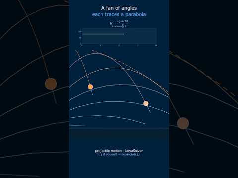
Range: $R = \frac{v_0^2 \sin 2\theta}{g}$
Maximum height: $H = \frac{v_0^2 \sin^2\theta}{2g}$
Flight time: $T = \frac{2v_0 \sin\theta}{g}$
Area under the v-t graph → displacement x
Slope of the v-t graph → acceleration a
With constant acceleration, v-t is a straight line and x-t is a parabola.
What is Kinematics?
🙋
What exactly is kinematics? Is it just about plugging numbers into formulas?
🎓
Basically, kinematics is the geometry of motion. It describes how things move—their position, velocity, and acceleration—without worrying about why they move (that's dynamics). In practice, the equations you see here are the mathematical toolkit for that description. Try moving the 'Initial Velocity' slider in the 1D section above and watch how the position-time graph changes instantly. That's kinematics in action.
🙋
Wait, really? So if I know the acceleration and initial speed, these equations can tell me everything? What's the catch?
🎓
The key catch is constant acceleration. These three famous equations only work when acceleration doesn't change. A common case is free fall near Earth's surface, where gravity provides a constant ~9.8 m/s² downward. For instance, if you throw a ball straight up, its acceleration is always -9.8 m/s², even at the top where its velocity is zero. Try setting acceleration to -9.8 in the simulator and see how velocity decreases linearly.
🙋
That makes sense for 1D. But the simulator also does 2D projectiles. How do those equations connect? Is it just two 1D motions glued together?
🎓
Exactly right! Projectile motion is the perfect example of superposition. The horizontal motion has zero acceleration (constant velocity), while the vertical motion has constant downward acceleration from gravity. They are independent. When you change the launch angle θ in the 2D panel, you're just splitting the initial velocity into horizontal ($v_0 \cos\theta$) and vertical ($v_0 \sin\theta$) components, then applying the 1D equations to each.
Physical Model & Key Equations
The core model assumes constant acceleration. The three equations form a complete set, allowing you to solve for any unknown kinematic variable if you know the others. They are derived from the definitions of velocity and acceleration.
Where $x_0$ is initial position (m), $v_0$ is initial velocity (m/s), $v$ is final velocity (m/s), $a$ is constant acceleration (m/s²), and $t$ is time elapsed (s).
For 2D projectile motion, we apply the constant-acceleration model separately to the x (horizontal) and y (vertical) axes. The only acceleration is gravity ($g$) acting downward. This leads to specific results for range and maximum height.
Here, $R$ is the total horizontal distance traveled (range), $H$ is the maximum height, $v_0$ is the initial launch speed, $\theta$ is the launch angle above the horizontal, and $g$ is the acceleration due to gravity (9.8 m/s² on Earth).
Frequently Asked Questions
You input velocity by drawing a straight line on the graph using a mouse or touch operation. The slope of the drawn line is automatically calculated as acceleration, and the area as displacement, which are visualized in real time. If you draw a curve instead of a straight line, it is interpreted as an approximated uniformly accelerated motion.
No, the projectile motion mode of this simulator assumes an ideal vacuum environment without air resistance. The horizontal direction is calculated as uniform linear motion, and the vertical direction as uniformly accelerated motion with only gravitational acceleration (-g). For cases including air resistance, please use a separate CAE tool.
Yes, all parameters can be set to negative values. For example, setting the initial velocity to a negative value represents motion in the opposite direction, and setting the initial position to a negative value represents starting from the left (or below) the origin. If the signs of acceleration and velocity differ, it is correctly visualized as decelerating motion.
Currently, there is no direct export function, but hovering the mouse over the graph in each mode displays the velocity, position, and acceleration for each time step numerically. Additionally, you can copy all displayed time-series data to the clipboard using the 'Copy Data' button at the bottom right of the screen.
Real-World Applications
Automotive Safety & Crash Testing: CAE software uses the fundamental principles of kinematics as a starting point for simulating vehicle collisions. While real crashes involve complex, changing forces, the constant-acceleration equations provide a first-order estimate of stopping distances and the forces occupants experience, which informs airbag deployment timing and crumple zone design.
Sports Science & Performance: Analyzing the trajectory of a basketball, soccer ball, or javelin is pure projectile motion. By understanding the relationship between launch angle, speed, and range, coaches and athletes can optimize techniques for maximum distance or accuracy, such as finding the ideal angle for a long throw-in.
Robotics & Trajectory Planning: For a robotic arm to move smoothly from point A to point B, its controller must plan a kinematic trajectory—defining its position, velocity, and acceleration at every moment in time. These constant-acceleration equations form the basis for simple, smooth motion profiles.
Structural Dynamics & Earthquake Engineering: The CAE link mentioned—the Newmark-β method—is a direct generalization of these kinematics equations. It solves for the displacement, velocity, and acceleration of complex structures (like buildings or bridges) over time when subjected to dynamic loads like earthquakes, using the same core concepts of relating these three quantities.
Common Misconceptions and Points to Note
First, note that it's easy to forget the assumption of "constant acceleration". This simulator deals with an ideal world where "acceleration is constant". For example, even if you press a car's accelerator steadily, the actual acceleration changes due to air resistance or road gradient. In practice, you should treat calculation results from this tool as a "rough guideline" and verify them with more detailed models.
Next, calculation errors due to mixed units are frequent. The simulator's input fields are primarily in [m/s] or [m/s²], but real-world data often comes in [km/h] or [G]. For instance, to input an initial velocity of 60 km/h, you must convert it to 60 ÷ 3.6 ≈ 16.7 m/s. This kind of unit conversion mistake can throw your result off by an order of magnitude, so get into the habit of always checking your units.
Finally, there is a common misunderstanding of overlooking the "launch and landing point heights" in 2D projectile motion. The simulator's default setting assumes the launch and landing points are at the same height (y=0), but for example, when throwing a ball off a cliff, the initial height $y_0$ is positive. This difference significantly affects the time of flight and range. If you experiment with the altitude parameter in the tool, you should be able to appreciate the magnitude of this effect.
Enter initial position (i_x0) in meters and initial velocity magnitude (i_v0) in m/s
Set launch angle using the input field (0–90°) or v0Slider for velocity components
Input acceleration (i_a) in m/s² and time interval (i_t) in seconds
Click Calculate to generate Range R, Maximum Height H, Flight Time, and trajectory visualization
Adjust parameters to see real-time graph updates showing position vs. time curves
Worked Example
A projectile launched at 25 m/s, 35° angle, from ground level (x0=0, y0=0). Gravity a=−9.81 m/s². Initial velocity components: vx=20.5 m/s, vy=14.3 m/s. Calculations yield: Range R=61.4 m, Maximum Height H=10.5 m, Flight Time=2.92 seconds. The simulator plots the parabolic arc and generates position tables at 0.5-second intervals, confirming peak height at t=1.46 s.
Practical Notes
For artillery or ballistics analysis, 45° angle maximizes range in level-ground scenarios; adjust for wind resistance by reducing v0 by 2–5%
Basketball shot analysis: typical launch angle 50–52° with v0=7.5 m/s from 2.1 m height yields H=3.8 m clearance
Use time-series output to validate kinematic equations: x(t)=x0+v0t+½at², especially for non-zero initial heights in drone or ramp problems
🎬 Watch it in motion
Projectile Motion | the safety parabola you can't beat #Shorts