Wear Simulation
Theory and Physics
What is Wear Simulation?
Professor, can we simulate wear (material loss) using FEM?
Yes. It calculates material removal on contact surfaces based on the Archard wear law and updates the geometry.
$V$ is wear volume, $s$ is sliding distance, $K$ is wear coefficient, $F_n$ is normal force, $H$ is hardness.
Wear is proportional to sliding distance. It's a simple model.
The Archard equation is the simplest, but provides practical accuracy for many wear problems.
Implementation in FEM
Wear simulation procedure (iterative):
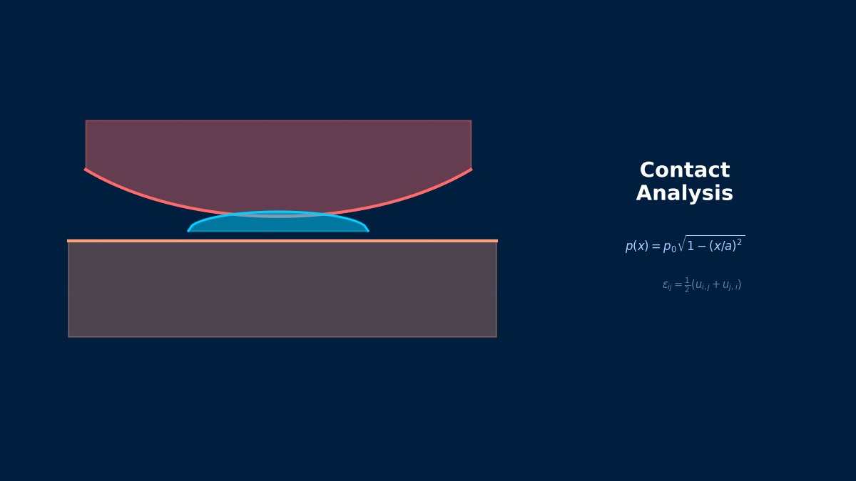
1. Contact Analysis — Calculate contact pressure and sliding amount
2. Wear Amount Calculation — Wear depth using Archard's equation
3. Mesh Update — Move nodes by the worn amount
4. Contact Analysis Again — With the updated geometry
5. Iterate until convergence
Updating the mesh each time seems tough.
Can be automated using Abaqus UMESHMOTION (adaptive meshing) or LS-DYNA *MAT_WEAR.
Summary
Key Points:
- Archard Wear Law — $dV/ds = K F_n / H$
- Iteration of Contact → Wear Amount → Mesh Update — Time evolution of wear
- Abaqus UMESHMOTION — Updates wear surface with adaptive mesh
- Bearings, Gears, Brake Pads — Main applications
Archard Wear Law 1953
The Archard wear law, which forms the basis of wear simulation, originates from a paper published by J.F. Archard and W. Hirst in 1953. It is a simple proportional law: wear volume V = k × W × s / H (k: wear coefficient, W: load, s: sliding distance, H: hardness). Even after over 60 years, it continues to be used as the standard model for industrial wear prediction. This paper preceded the launch of the Wear journal (1957) and greatly contributed to the establishment of the academic field of tribology.
Physical Meaning of Each Term
- Inertia Term (Mass Term): $\rho \ddot{u}$, i.e., "mass × acceleration". Have you ever experienced being thrown forward during sudden braking? That "feeling of being pulled" is precisely the inertial force. Heavier objects are harder to set in motion and harder to stop once moving. Buildings shake during earthquakes because the ground moves suddenly while the building's mass is "left behind". In static analysis, this term is set to zero, which assumes "forces are applied slowly so acceleration can be ignored". It absolutely cannot be omitted for impact loads or vibration problems.
- Stiffness Term (Elastic Restoring Force): $Ku$ or $\nabla \cdot \sigma$. When you stretch a spring, you feel a "force trying to return it", right? That is Hooke's law $F=kx$, the essence of the stiffness term. Now a question—if you pull an iron rod and a rubber band with the same force, which stretches more? Obviously the rubber. This "resistance to stretching" is the Young's modulus $E$, which determines stiffness. A common misconception: "high stiffness = strong" is incorrect. Stiffness is "resistance to deformation", strength is "resistance to failure"—they are different concepts.
- External Force Term (Load Term): Body force $f_b$ (gravity, etc.) and surface force $f_s$ (pressure, contact force, etc.). Think of it this way—the weight of a truck on a bridge is a "force acting on the entire volume" (body force), while the force of the tire pushing on the road is a "force acting only on the surface" (surface force). Wind pressure, water pressure, bolt tightening force... all are external forces. A typical mistake here: getting the load direction wrong. Intending "tension" but ending up with "compression"—it sounds like a joke, but it actually happens when coordinate systems are rotated in 3D space.
- Damping Term: Rayleigh damping $C\dot{u} = (\alpha M + \beta K)\dot{u}$. Try plucking a guitar string. Does the sound continue forever? No, it gradually fades away. That's because vibration energy is converted to heat by air resistance and internal friction in the string. Car shock absorbers work on the same principle—they intentionally absorb vibration energy to improve ride comfort. What if damping were zero? Buildings would keep shaking forever after an earthquake. Since that doesn't happen in reality, setting appropriate damping is crucial.
Assumptions and Applicability Limits
- Continuum assumption: Treats material as a continuous medium, ignoring microscopic inhomogeneity
- Small deformation assumption (for linear analysis): Deformation is sufficiently small compared to initial dimensions, stress-strain relationship is linear
- Isotropic material (unless specified otherwise): Material properties are independent of direction (anisotropic materials require separate tensor definition)
- Quasi-static assumption (for static analysis): Ignores inertial/damping forces, considers only balance between external and internal forces
- Non-applicable cases: For large deformation/large rotation problems, geometric nonlinearity is required. For plasticity, creep, and other nonlinear material behaviors, constitutive law extension is needed
Dimensional Analysis and Unit Systems
| Variable | SI Unit | Notes / Conversion Memo |
|---|---|---|
| Displacement $u$ | m (meter) | When inputting in mm, unify loads/elastic modulus to MPa/N system |
| Stress $\sigma$ | Pa (Pascal) = N/m² | MPa = 10⁶ Pa. Be careful of unit inconsistency when comparing with yield stress |
| Strain $\varepsilon$ | Dimensionless (m/m) | Note the distinction between engineering strain and logarithmic strain (for large deformation) |
| Elastic Modulus $E$ | Pa | Steel: ~210 GPa, Aluminum: ~70 GPa. Note temperature dependence |
| Density $\rho$ | kg/m³ | In mm system: tonne/mm³ (= 10⁻⁹ tonne/mm³ for steel) |
| Force $F$ | N (Newton) | Unify as N in mm system, N in m system |
Numerical Methods and Implementation
FEM Implementation of Wear
```
*ADAPTIVE MESH, TYPE=CONTACT SURFACE
wear_surface
*ADAPTIVE MESH CONTROLS, MESHING FREQUENCY=1
*UMESHMOTION $ Calculate wear amount in user subroutine
```
```
*MAT_WEAR
K, H $ Archard coefficient and hardness
```
So LS-DYNA has a dedicated wear material model.
*MAT_WEAR automatically thins contact surface elements to represent wear. Wear progresses without remeshing.
Summary
Numerical Scheme for Geometry Update
The numerical core of wear FEM lies in the iterative process of "wear amount → node movement → mesh update → re-contact". In the Eulerian approach proposed by Podra & Andersson (1997), the wear amount for one cycle is calculated using the Archard law, boundary nodes are retracted in the normal direction, and then element distortion is corrected using a smoothing algorithm. This method is still referenced as a reference implementation for ABAQUS UMESHMOTION user subroutine implementations.
Linear Elements (1st Order Elements)
Linear interpolation between nodes. Low computational cost but low stress accuracy. Beware of shear locking (mitigated with reduced integration or B-bar method).
Quadratic Elements (with Mid-side Nodes)
Can represent curved deformation. Stress accuracy improves significantly, but degrees of freedom increase by about 2-3 times. Recommended: when stress evaluation is critical.
Full Integration vs Reduced Integration
Full Integration: Risk of over-constraint (locking). Reduced Integration: Risk of hourglass mode (zero-energy mode). Choose appropriately.
Adaptive Mesh
Automatic refinement based on error indicators (e.g., ZZ estimator). Efficiently improves accuracy in stress concentration areas. Includes h-method (element subdivision) and p-method (order increase).
Newton-Raphson Method
Standard method for nonlinear analysis. Updates tangent stiffness matrix each iteration. Quadratic convergence within convergence radius, but high computational cost.
Modified Newton-Raphson Method
Updates tangent stiffness matrix from initial value or every few iterations. Cost per iteration is low, but convergence speed is linear.
Convergence Criteria
Force residual norm: $||R|| / ||F_{ext}|| < \epsilon$ (typically $\epsilon = 10^{-3}$〜$10^{-6}$). Displacement increment norm: $||\Delta u|| / ||u|| < \epsilon$. Energy norm: $\Delta u \cdot R < \epsilon$
Load Increment Method
Applies full load not at once but in small increments. The arc-length method (Riks method) can trace beyond extremum points on the load-displacement curve.
Analogy: Direct Method vs Iterative Method
The direct method is like "solving simultaneous equations accurately with pen and paper"—reliable but takes too long for large-scale problems. The iterative method is like "repeatedly guessing to approach the correct answer"—starts with a rough answer but accuracy improves with each iteration. It's the same principle as looking up a word in a dictionary: it's more efficient to estimate where to open it and adjust forward/backward (iterative method) than to search sequentially from the first page (direct method).
Relationship Between Mesh Order and Accuracy
1st order elements are like "approximating a curve with a ruler"—represented by straight line segments, so accuracy is limited. 2nd order elements are like a "flexible curve"—can represent curved changes, dramatically improving accuracy even at the same mesh density. However, computational cost per element increases, so judge based on total cost-effectiveness.
Practical Guide
Wear in Practice
Practical Checklist
Cutting Tool Wear Prediction
FEM incorporating the Archard wear law for metal cutting tool life prediction has become widespread since the 2000s. In an analysis of carbide end mills published by Sandvik in the 2010s using the DEFORM code, the machining length until tool flank wear width VB=0.3mm was predicted under conditions of cutting speed 200m/min and depth of cut 1mm, with an error of ±18% compared to experimental values. This result is used for design decisions in tool coating optimization.
Analogy: Analysis Flow
The analysis flow is actually very similar to cooking. First, buy ingredients (prepare CAD model), do the prep work (mesh generation), apply heat (solver execution), and finally plate it (visualization in post-processing). Here's an important question—which step is most prone to failure in cooking? Actually, it's the "prep work". If mesh quality is poor, the results will be a mess no matter how good the solver is.
Pitfalls Beginners Often Fall Into
Are you checking mesh convergence? Do you think "the calculation ran = the result is correct"? This is actually the most common trap for CAE beginners. The solver will always return "some answer" for the given mesh. But if the mesh is too coarse, that answer is far from reality. Confirm that results stabilize with at least three levels of mesh density—neglecting this leads to the dangerous assumption that "the computer gave the answer, so it must be correct".
Thinking About Boundary Conditions
Setting boundary conditions is the same as "writing the exam question". If the question is wrong? No matter how accurately you calculate, the answer will be wrong. "Is this surface really fully fixed?" "Is this load really uniformly distributed?"—Correctly modeling real-world constraint conditions is actually the most important step in the entire analysis.
Software Comparison
Wear Tools
Selection Guide
Related Topics
なった
詳しく
報告