Near-Field Electromagnetic Coupling Analysis
Near-Field Electromagnetic Coupling Analysis: Theoretical Foundations
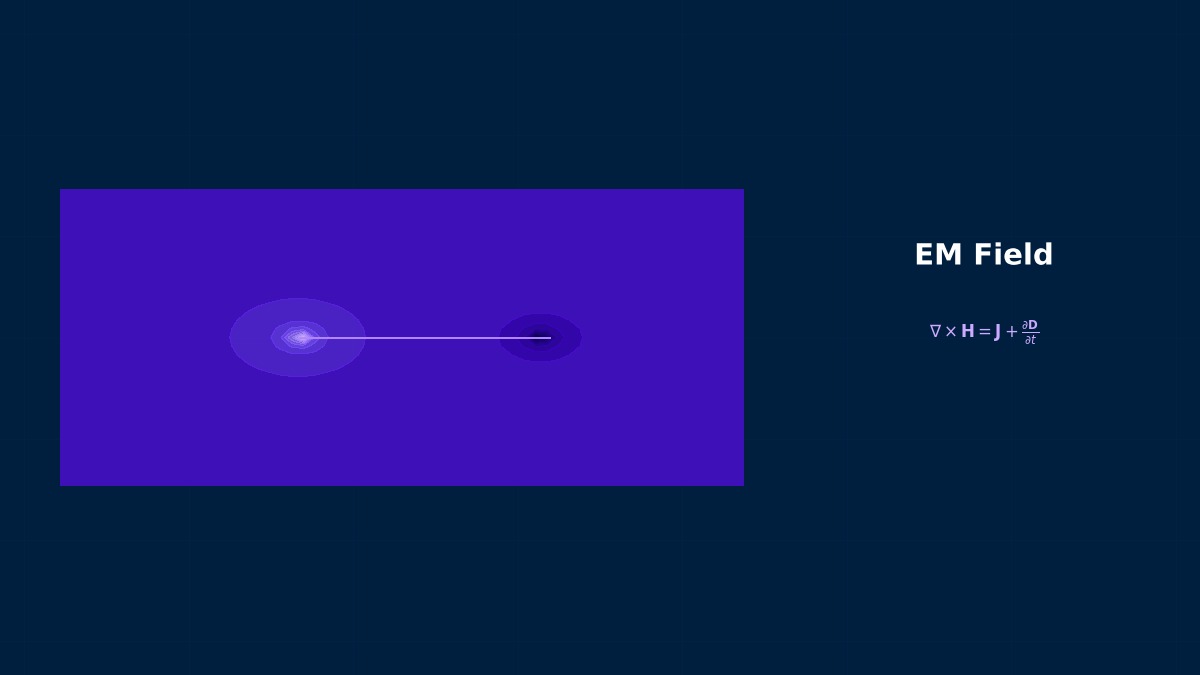
Overview
Professor! Today's topic is about near-field coupling analysis, right? What exactly is it?
Numerical analysis of magnetic field coupling and electric field coupling between circuits/wires. Extraction of mutual inductance and mutual capacitance. Printed circuit board layout optimization.
Your explanation is easy to understand! The fog around magnetic field coupling between circuits and wires has cleared up.
Governing Equations
I see... Describing near-field coupling analysis seems simple at first glance, but it's actually very profound, isn't it?
Discretization Methods
How do you actually solve these equations on a computer?
We use spatial discretization by the Finite Element Method (FEM). We assemble the element stiffness matrix and construct the global stiffness equation.
We perform transformation to the weak form (variational form) and use formulation by the Galerkin method using test functions and shape functions. The choice of element type (low-order elements vs. high-order elements, full integration vs. reduced integration) directly affects the trade-off between solution accuracy and computational cost.
Matrix Solution Algorithms
What exactly do you mean by matrix solution algorithms?
Solve the simultaneous equations using direct methods (LU decomposition, Cholesky decomposition) or iterative methods (CG method, GMRES method). For large-scale problems, preconditioned iterative methods are effective.
| Solver | Classification | Memory Usage | Applicable Scale |
|---|---|---|---|
| LU decomposition | Direct Method | O(n²) | Small to Medium Scale |
| Cholesky decomposition | Direct Method (Symmetric Positive Definite) | O(n²) | Small to Medium Scale |
| PCG Method | Iterative Method | O(n) | Large Scale |
| GMRES method | Iterative Method | O(n·m) | Large Scale / Non-symmetric |
| AMG Preconditioner | Preprocessing | O(n) | Very Large Scale |
So, if you cut corners on the finite element method part, you'll pay for it later. I'll keep that in mind!
Implementation in Commercial Tools
So, what software can be used to do near-field coupling analysis?
| Tool Name | Developer/Current Status | Main File Format |
|---|---|---|
| CST Studio Suite | Dassault Systèmes SIMULIA | .cst |
| Ansys HFSS | Ansys Inc. | .aedt, .hfss |
| COMSOL Multiphysics | COMSOL AB | .mph |
Vendor Lineage and Product Integration History
Is the origin story of each software quite dramatic?
CST Studio Suite
What exactly is CST Studio?
Developed by Computer Simulation Technology (Germany). Acquired by Dassault Systèmes in 2016 and integrated into SIMULIA.
Current Affiliation: Dassault Systèmes SIMULIA
Ansys HFSS
Next is the story about Ansys HFSS. What's it about?
A 3D high-frequency electromagnetic field simulator developed by Ansoft Corporation. Ansys acquired Ansoft in 2008.
Current Affiliation: Ansys Inc.
COMSOL Multiphysics
Please tell me about "COMSOL Multiphysics"!
Founded in Sweden in 1986. Started as FEMLAB with MATLAB integration, later renamed to COMSOL. Strong in multiphysics.
Current Affiliation: COMSOL AB
So, if you cut corners on the German part, you'll pay for it later. I'll keep that in mind!
File Formats and Interoperability
Are there any points to note when transferring data between different software?
| Format | Extension | Type | Overview |
|---|---|---|---|
| STEP | .stp/.step | Neutral CAD | 3D CAD data exchange format compliant with ISO 10303. Supports geometry + PMI. |
| IGES | .igs/.iges | Neutral CAD | Early CAD data exchange standard. Has issues with surface data compatibility. Transition to STEP is progressing. |
| STL | .stl | Mesh | Triangular facets only. 3D printer standard. Not suitable for CAE meshes. |
When converting models between different solvers, attention must be paid to the correspondence of element types, compatibility of material models, and differences in the representation of loads/boundary conditions. Particularly, high-order elements and special elements (cohesive elements, user-defined elements, etc.) often cannot be directly converted between solvers.
I see... Formats seem simple at first glance, but they're actually very profound, aren't they?
Practical Considerations
Are there things like "field wisdom" that aren't written in textbooks?
Verifying mesh convergence, validating the appropriateness of boundary conditions, and performing sensitivity analysis of material parameters are extremely important.
- Mesh Dependency Verification: Confirm convergence with at least 3 levels of mesh density.
- Boundary Condition Validity: Setting physically meaningful constraint conditions.
- Result Verification: Comparison with theoretical solutions, experimental data, and known benchmark problems.
Yeah, you're on the right track! Actually getting your hands dirty is the best way to learn. If you don't understand something, feel free to ask anytime.
Near Field and Far Field—The "Boundary" is Determined by λ/2π
The boundary between the "near field" and "far field" of electromagnetic waves is approximately at a distance of r = λ/(2π) (about 1/6 of the wavelength). Within this boundary, the ratio of electric field to magnetic field (wave impedance) varies greatly between 37 and 377 Ω, and the simple plane wave approximation does not hold. For high-speed signals on PCBs and cables, the wavelength is around 30 cm at several hundred MHz, and the distance to adjacent boards often falls within the near-field region. The ability to accurately simulate this "complex near-field coupling" is one of the values of modern EMC analysis.
Related Topics
Experience the theory firsthand with the interactive simulator for this field
All Simulators